Download
1 / 44
440 likes | 591 Views
Super flat IR beam pipe. Super B Factory WS in Hawaii Jan. 22, 2004 Hidekazu Kakuno (TIT) Hitoshi Ozaki & Nobu Katayama (KEK). Outline. Motivation Super flat geometry Simulation method Simulation results Vertexing and B/D separation B s – B s mixing parameter measurement

E N D
Super flat IR beam pipe Super B Factory WS in Hawaii Jan. 22, 2004 Hidekazu Kakuno (TIT) Hitoshi Ozaki & Nobu Katayama (KEK)
Outline • Motivation • Super flat geometry • Simulation method • Simulation results • Vertexing and B/D separation • Bs – Bs mixing parameter measurement • B Dtn branching fraction measurement • Issues and conclusions H.Kakuno, H. Ozaki & N. Katayama
Single B samples • It’s been discussed that many interesting measurements require “single B event” samples • B Knn • B tn,Bstt • B Dtn • b uln and other inclusive measurements • … H.Kakuno, H. Ozaki & N. Katayama
B reconstruction at U(4S) • At B factories we can identify (reconstruct) only much less than 1% of the actual B decays. This is because • B has many decay modes, and D has many decay modes • Average multiplicity of the B decay is 5~6 charged, 3 neutral • Lots of combinatorial backgrounds • Combinatorial background can be reduced using topologicalinformation on tracks (combinations) • Continuum backgrounds as well (ccbar for BD and uds for non-charm decays) H.Kakuno, H. Ozaki & N. Katayama
Standard Vertex Resolution • Thickness of the material before the first measurement ~1mm (Au/Ag + Be + Si + …) • Distance between the vertices and the first measurements minimum 2~3 cm • Resolution of the first measurement 7~30mm dX, dZ : 80~100 mm (dY:20mm IP profile + B flight length) • Solid angle coverage of the first measurements ~92% H.Kakuno, H. Ozaki & N. Katayama
Super Vertexing • If the error in the vertex measurement, sz were less than 10 mm, it helps in doing • B reconstruction • We can separate B, Bbar, D and Dbar vertices, we can greatly reduce the combinatorial and continuum background and identify many B decays • Continuum separation • Measurements of some decays such as B Dtn • Reconstruct momentum vector using two vertices • Bs – Bs mixing measurements; even for X>15 H.Kakuno, H. Ozaki & N. Katayama
B Dtn reconstruction n D t B IP profile n • IP profile + D direction B vertex • B vertex + t vertex (helix ext.) + t mass t momentum (and the entire t kinematics): 0c-fit • Make missing mass of the nt from B • Lots of combinatorial backgrounds but measure Br. without full B reconstruction tag H.Kakuno, H. Ozaki & N. Katayama
Bstt reconstructions n n t t B IP profile • Much more difficult as we cannot measure the B decay vertex • IP profile + 2 t vertex (helix ext.) + 2 t mass B vertex (and the entire t kinematics): 0c-fit • Or + vertex of the other B to get Vx: 1c-fit H.Kakuno, H. Ozaki & N. Katayama
Super flat geometry • Make first measurements as close to IP as possible • Follow the flat beam profile (times >100 sigmas) • Flat because silicon wafer is flat (without thinning) • Sort of ideal geometry for physics • Machine issues not seriously considered • Keep hermeticity similar to what we have now (90% of 4p) • Geometry is not optimized (yet) H.Kakuno, H. Ozaki & N. Katayama
IP profile • B factories have proven b*y ~ 5 mm and bunch length of 5mm are possible • For Super B factories, the parameters have been aggressively pushed to: 3mm and 3mm giving IP beam size of sy< 2mm • sy is said to be limited by beam-beam effects • Due to X-Y coupling, sy is also affected by b*x • IR beam pipe can be as small (and short) as the size of beams (times clearance, say, 100 sigmas) H.Kakuno, H. Ozaki & N. Katayama
Super KEKB beamparameters • Assuming XY coupling of 5% • sz ~ 3 mm • Maybe parameters are somewhat old H.Kakuno, H. Ozaki & N. Katayama
Cross section of the S-F beam pipe Silicon vertex detector (300mm thick) Vacuum y Beryllium beam pipe (500mm) x 10 mm 1 mm Cooling H.Kakuno, H. Ozaki & N. Katayama
Top view of the S-F beam pipe Z (boost) Detector length Cone for 17° Pixel Detector ±2.5 cm is Enough! 1.6 cm 1cm Cone for 30° 1.4cm H.Kakuno, H. Ozaki & N. Katayama Sensitive region is 1.4cm wide
Side view of S-F beam pipe Vacuum or accelerator components (nano beta??) Silicon vertex detector (300mm thick) Beryllium beam pipe(500mm) 1.6 cm H.Kakuno, H. Ozaki & N. Katayama
Study of the S-F beam pipe • Using Geant4 we defined the S-F geometry; vacuum and beam pipe @IP and the silicon vertex detector • In BelleG4, the event generator information written in Belle format is read in. • After propagating the tracks in the above geometry, momentum and position of the tracks at r=2cm as well as hits on the silicon vertex detector are written out • The silicon hits are smeared using DSSD intrinsic resolution • sigma = 5 + 10.65*alpha (alpha in rad) for both Z and f • We then process the tracks (track by track trackerr) using the Belle SVD 1.x + old CDC geometry (100% effic) Outer SVD resolution used in simulation Z (inner/outer layer) rf inner/outer layer • Explicit Kalman filter is applied to the inner silicon hits and multiple scattering in the silicln and beam pipe materials • The tracks have been extrapolated at the vertex using IP constraint (y=0) H.Kakuno, H. Ozaki & N. Katayama
BD*ln + BbarDtn H.Kakuno, H. Ozaki & N. Katayama
Inefficiency (no SVD hit) due to the above flat geometry is about 10% (1.4cm sensitive Region) for single track H.Kakuno, H. Ozaki & N. Katayama
1 mm H.Kakuno, H. Ozaki & N. Katayama
dr and dZ resolution at the vertex p=1GeV/c muon <20mm l(deg) l(deg) <30mm <20mm <10mm <10mm f(deg) f(deg) d(dZ) d(dr) H.Kakuno, H. Ozaki & N. Katayama
Background reduction Dkpw/wo vertex fit (no PID) • By requiring a good vertex (prob.<1%), backgrounds become 1/3 with 1% signal reduction • first Si hit for both tracks • no. of CDC hits >20 for both tracks • 17 < theta < 150 deg. for both tracks • pt > 50 MeV/c for both tracks • IP info is not used in vertexing • With primary, B and D/t vertices separated cleanly, combinatorial and continuum backgrounds cangreatly be reduced H.Kakuno, H. Ozaki & N. Katayama
One BDpp, D Kpp H.Kakuno, H. Ozaki & N. Katayama
B+D-p+p+,D-K+p-p-, resolution study (1) • D- vertexing efficiency and resolution • All three (K+p-p-) tracks are to have • CDC hits > 20 • 17 < theta < 150deg; pt > 50 MeV/c • If all three tracks hit the first SVD, use them for vertexing, if one misses, use the other two tracks • vertexing efficiency = 96.9 0.2% • resolution ~10mm H.Kakuno, H. Ozaki & N. Katayama
B+D-p+p+,D-K+p-p-, resolution study (2) • B+ vertexing efficiency • Both (p+p+) tracks are to have • CDC hits > 20 • 17 < theta < 150deg; pt > 50 MeV/c • If both tracks hit the first SVD, use them for vertexing, if one misses, use the other track and IP profile • vertexing efficiency: 98.60.2% • resolution ~10mm H.Kakuno, H. Ozaki & N. Katayama
D flight distance from B decay No degradation!! Mean 310mm Measured (mm) Generated (mm) H.Kakuno, H. Ozaki & N. Katayama
S-F geometry vs current geom. Error on flight distance (mm) Error on flight distance (mm) See difference in scale H.Kakuno, H. Ozaki & N. Katayama
Separating B and D with L/dL • Using a flight length cut (L/dL) we can separate B and D vertecies • With S-F beam pipe, the separation is 4~5 times better Current geometry Cut S-F geometry Significance (L/dL) Better H.Kakuno, H. Ozaki & N. Katayama
Bs – Bs mixing • With S-F geometry, resolution is good enough to observe Bs – Bs mixing • We have generated events with X=15 for about 30 fb-1 of U(5S) running • DZ distribution using generator information H.Kakuno, H. Ozaki & N. Katayama
Analysis using dileptons • two same sign leptons (opposite sign events not used) • p(lepton) > 1 GeV/c (for clean lepton ID) • both lepton hit SVD 1st layer • 30<theta<150 deg to reject bad z resolution region • p*(lepton) > 1.2 GeV/c to reject 2nd lepton from charm H.Kakuno, H. Ozaki & N. Katayama
DZ resolution andDZ distributions with dZ cuts Expected DZ distribution Gen Meas/no cut 30mm 40mm 50mm Residual(Measured – generated) 30mm 20mm FWHM/2.36~27mm H.Kakuno, H. Ozaki & N. Katayama
Results and comments • s(U(5S)) ~ 0.27 nb • Fraction of Bs: 0.263(Bs*Bs*), 0.022(Bs*Bs), 0.046(BsBs) (L=odd dominant, an estimation) • We have not done fits but, • It seems we can easily observe mixing if X=15 with a few tens of fb-1 @ 5S with the super flat beam pipe. Considering the vertex resolution, we can go up to X=20 • Note that we have not added other same sign dilepton backgrounds H.Kakuno, H. Ozaki & N. Katayama
Analysis using D*ln + B anything • D* Dp Kp/K3p vertexing with nominal D mass and D* - D mass difference cuts • Signal side B vertex using D, l, and IP • Standard Belle tagging + vertrxing for the tag side • For now generator information is used to select combinations • We generated 105 Bd - Bd events with X=15 • We generated assuming sy=15mm. In super B design it is 2mm. Although smearing due to B flight length dominates (20mm) results will be slightly worse than it could be in the following analyses H.Kakuno, H. Ozaki & N. Katayama
Vertex resolutions s=28mm, Offset:14mm s=13mm H.Kakuno, H. Ozaki & N. Katayama
Results • We can clearly see oscillation as well • 105 events is ~6fb-1 at U(5S) H.Kakuno, H. Ozaki & N. Katayama
B Dtn analysis • Reconstruct D Kp and t 3p, extrapolate D momentum vector from D vertex, make B vertex using IP, use the B vertex and t vertex to calculate t direction, calculate t momentum using t mass constraint • Problem: t 3p has lots of combinatorial background even in signal (with the other B decaying generically) Monte Carlo sample • We use tight cuts for vertexing and flight length cuts requiring separation of vertices H.Kakuno, H. Ozaki & N. Katayama
B, Btag and t vertex separation The best candidate in a event is selected using sum of c2 for the vertex fits True Dtn Wrong Dtn H.Kakuno, H. Ozaki & N. Katayama
B Dtn missing mass C = 2×p*Dt×p*B cosq = MM2/C Solid: this method Dotted: with generated t direction H.Kakuno, H. Ozaki & N. Katayama
Pt and mnt reconstruction Using the rest of event Solid: this method Dotted: generated t momentum after MM2 cut H.Kakuno, H. Ozaki & N. Katayama
Efficiencies (cumulative) H.Kakuno, H. Ozaki & N. Katayama
Results S/N = 2427/264 ~ 10 where N is combinatorial background in signal MC • Need to estimate background from generic B decays • Using D*ln+generic (D*ln+D*ln) sample, treating l as p, we see 8(7) events in 100,000 samples • As we know all kinematical info for t 3pn we can compute t polarization as well H.Kakuno, H. Ozaki & N. Katayama
Prospects • Br(B D tn) 1% • Br(D final) ~10% (averaging D0 and D+) (D0 Kp, K3p D+ K2p...) • Br(t 3pn) 10% • Efficiency: 2% • Number of reconstructed signals = 0.01 × 0.1 × 0.1 × 0.02 × 2 × 106 / fb-1 = 4 events / fb-1 = 4k events / ab-1 (<200 / ab-1for full recon. tag method) • We can observe B Dtn and measure polarization “without full reconstruction”! H.Kakuno, H. Ozaki & N. Katayama
Difficulties/Further studies • Beam clearance • Accidental damage • Image current: assume r = 0.5mm round bp (Yamamoto) • r = 0.5mm, l = 2cm, Ibeam = 10amp.(LER) • bunch spacing = 0.6m, bunch-length(sz) = 3mm. • total Wattage = 1.0 KW(LER) + 0.25KW(HER) • HOM • Noise • Backgrounds • … H.Kakuno, H. Ozaki & N. Katayama
Conclusions • A simulation-reconstruction-analysis chain has established using new (?) tools • The S-F beam pipe geometry has been implemented in a simulation program using Geant4 and Belle data format • A track-by-track version of trackerr has been implemented in Belle framework • A Kalman filter has been implemented for the S-F beam pipe geometry • If we can separate (most of) B and D (and other) vertices in an event, the B reconstruction and flavor tagging techniques will dramatically be improved • Need more studies • Bs-Bsbar mixing possible @U(5S) • New way of reconstruction technique is possible • Use two vertices to obtain direction of momentum vector H.Kakuno, H. Ozaki & N. Katayama
Conclusions • We need to investigate feasibility of the S-F beam pipe with the accelerator group • The round beam pipe design may have limitation in making the first measurements as close as possible for the current flat beam profile. We can either go to round beams or flat beam pipe • If the bunch length can be shorter, the flat beam pipe can be shorter • L = 2~3*sz+60*sy+3 mm • The shorter the beam pipe the smaller heating will be • SF beam pipe is very cheap, compared with the machine upgrade to get high luminosity to achieve the same “luminosity×efficiency” for many analyses H.Kakuno, H. Ozaki & N. Katayama
History of beam pipe radius 1mm@ 2010! H.Kakuno, H. Ozaki & N. Katayama