Download
1 / 36
360 likes | 451 Views
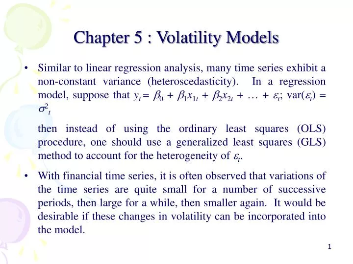
Chapter 5 : Volatility Models. Similar to linear regression analysis, many time series exhibit a non-constant variance (heteroscedasticity). In a regression model, suppose that y t = 0 + 1 x 1 t + 2 x 2 t + … + t ; var( t ) = 2 t

E N D
Chapter 5 : Volatility Models • Similar to linear regression analysis, many time series exhibit a non-constant variance (heteroscedasticity). In a regression model, suppose that yt = 0 + 1x1t + 2x2t + … + t; var(t) = 2t • then instead of using the ordinary least squares (OLS) procedure, one should use a generalized least squares (GLS) method to account for the heterogeneity of t. • With financial time series, it is often observed that variations of the time series are quite small for a number of successive periods, then large for a while, then smaller again. It would be desirable if these changes in volatility can be incorporated into the model.
This plot shows the weekly dollar/sterling exchange rate from January 1980 to December 1988 (470 observations)
The levels exhibit wandering movement of a random walk, and consistent with this, the differences are stationary about zero and show no discernable pattern, except that the differences tend to be clustered (large changes tend to be followed by large changes and small changes tend to be followed by small changes) • An examination of the series’ ACF and PACF reveals some of the cited characteristics
The ARIMA Procedure Name of Variable = rates Period(s) of Differencing 1 Mean of Working Series -0.00092 Standard Deviation 0.02754 Number of Observations 469 Observation(s) eliminated by differencing 1 Autocorrelations Lag Covariance Correlation -1 9 8 7 6 5 4 3 2 1 0 1 2 3 4 5 6 7 8 9 1 Std Error 0 0.00075843 1.00000 | |********************| 0 1 -0.0000487 -.06416 | .*| . | 0.046176 2 6.52075E-6 0.00860 | . | . | 0.046365 3 0.00005996 0.07906 | . |** | 0.046369 4 0.00004290 0.05657 | . |*. | 0.046655 5 -0.0000173 -.02284 | . | . | 0.046801 6 2.67563E-6 0.00353 | . | . | 0.046825 7 0.00006114 0.08061 | . |** | 0.046826 8 -9.5206E-6 -.01255 | . | . | 0.047121 9 6.54731E-6 0.00863 | . | . | 0.047128 10 0.00003322 0.04380 | . |*. | 0.047131 11 -0.0000507 -.06689 | .*| . | 0.047218 12 0.00001356 0.01788 | . | . | 0.047419 13 0.00001637 0.02158 | . | . | 0.047434 14 0.00003604 0.04752 | . |*. | 0.047455 15 1.26289E-6 0.00167 | . | . | 0.047556 16 0.00002185 0.02881 | . |*. | 0.047556 17 3.2823E-7 0.00043 | . | . | 0.047593 18 -0.0000340 -.04483 | .*| . | 0.047593 19 0.00005576 0.07352 | . |*. | 0.047683 20 5.5947E-6 0.00738 | . | . | 0.047924 21 -3.8865E-6 -.00512 | . | . | 0.047927 22 0.00001112 0.01466 | . | . | 0.047928 23 -0.0000168 -.02212 | . | . | 0.047938 24 0.00003914 0.05161 | . |*. | 0.047959 "." marks two standard errors
Partial Autocorrelations Lag Correlation -1 9 8 7 6 5 4 3 2 1 0 1 2 3 4 5 6 7 8 9 1 1 -0.06416 | .*| . | 2 0.00450 | . | . | 3 0.08023 | . |** | 4 0.06742 | . |*. | 5 -0.01626 | . | . | 6 -0.00704 | . | . | 7 0.07182 | . |*. | 8 -0.00271 | . | . | 9 0.00843 | . | . | 10 0.03316 | . |*. | 11 -0.07116 | .*| . | 12 0.01058 | . | . | 13 0.01856 | . | . | 14 0.05192 | . |*. | 15 0.01636 | . | . | 16 0.02016 | . | . | 17 -0.01202 | . | . | 18 -0.04319 | .*| . | 19 0.06369 | . |*. | 20 0.01375 | . | . | 21 0.00007 | . | . | 22 0.00120 | . | . | 23 -0.03788 | .*| . | 24 0.05154 | . |*. |
Engle (1982, Econometrica) called this form of heteroscedasticity, where 2t depends on 2t1, 2t2, 2t3, etc. “autoregressive conditional heteroscedasticity (ARCH)”. More formally, the model is where represents the past realized values of the series. Alternatively we may write the error process as
This equation is called an ARCH(q) model. We require that 0 > 0 and i≥ 0 to ensure that the conditional variance is positive. Stationarity of the series requires that
Typical stylized facts about the ARCH(q) process include: {t} is heavy tailed, much more so than the Gaussian White noise process. Although not much structure is revealed in the correlation function of {t}, the series {t2} is highly correlated. Changes in {t} tends to be clustered.
As far as testing is concerned, there are many methods. Three simple approaches are as follows: Time series test. Since an ARCH(p) process implies that {t2} follows an AR(p), one can use the Box-Jenkins approach to study the correlation structure of t2 to identify the AR properties Ljung-Box-Pierce test
Lagrange multipler test H0: 1 = 2 = … q = 0 H1: 1 ≥ 0, i = 1, …, q (with at least one inequality) To conduct the test, Regress et2 on its lags depends on the assumed order of the ARCH process. For an ARCH(q) process, we regress et2 on e2t1… e2tq. The LM statistic is under H0, where R2 is the coefficient of determination from the auxiliary regression.
The following SAS program estimates an ARCH model for the monthly stock returns of Intel Corporation from January 1973 to December 1977 • data intel; • infile'd:\teaching\ms6217\m-intc.txt'; • input r t; • r2=r*r; • lr2=lag(r2); • procreg; • model r2=lr2; • procarima; • identifyvar=r nlag=10; • run; • procarima; • identifyvar=r2 nlag=10; • run; • procautoreg; • model r= /garch =(q=4); • run; • procautoreg; • model r= /garch =(q=1); • outputout=out1 r=e; • run; • procprintdata=out1; • var e; • run;
The REG Procedure • Model: MODEL1 • Dependent Variable: r2 • Analysis of Variance • Sum of Mean • Source DF Squares Square F Value Pr > F • Model 1 0.01577 0.01577 9.53 0.0022 • Error 297 0.49180 0.00166 • Corrected Total 298 0.50757 • Root MSE 0.04069 R-Square 0.0311 • Dependent Mean 0.01766 Adj R-Sq 0.0278 • Coeff Var 230.46618 • Parameter Estimates • Parameter Standard • Variable DF Estimate Error t Value Pr > |t| • Intercept 1 0.01455 0.00256 5.68 <.0001 • lr2 1 0.17624 0.05710 3.09 0.0022
H0: 1 = 0 H1: otherwise LM = 299(0.0311) = 9.2989 > 21, 0.05 = 3.84 Therefore, we reject H0
The ARIMA Procedure • Name of Variable = r • Mean of Working Series 0.028556 • Standard Deviation 0.129548 • Number of Observations 300 • Autocorrelations • Lag Covariance Correlation -1 9 8 7 6 5 4 3 2 1 0 1 2 3 4 5 6 7 8 1 Std Error • 0 0.016783 1.00000 | |********************| 0 • 1 0.00095235 0.05675 | . |*. | 0.057735 • 2 -0.0000497 -.00296 | . | . | 0.057921 • 3 0.00098544 0.0587 | . |*. | 0.057921 • 4 -0.0005629 -.03354 | .*| . | 0.058119 • 5 -0.0007545 -.04496 | .*| . | 0.058184 • 6 0.00038362 0.0228 | . | . | 0.058299 • 7 -0.0002817 -.00678 .*| . | 0.058329 • 8 -0.0006309 -.03759 | .*| . | 0.059918 • 9 -0.0009289 -.05535 | .*| . | 0.059996 • 10 0.00097606 0.05816 | . |*. | 0.060166 • "." marks two standard errors
Generalized Autoregressive Conditional Heteroscedasticity (GARCH) The first empirical application of ARCH models was done by Engle (1982, Econometrica) to investigate the relationship between the level and volatility of inflation. It was found that a large number of lags was required in the variance functions. This would necessitate the estimation of a large number of parameters subject to inequality constraints. Using the concept of an ARMA process. Bollerslev (1986, Journal of Econometrics) generalized Engle’s ARCH model and introduced the GARCH model.
Specifically, a GARCH model is defined as with 0 > 0, i≥ 0, i =1, … q, j≥ 0, j = 1, … p imposed to ensure that the conditional variances are positive.
Usually, we only consider lower order GARCH processes such as GARCH (1, 1), GARCH (1, 2), GARCH (2, 1) and GARCH (2, 2) processes For a GARCH (1, 1) process, for example the forecasts are
Other diagnostic checks: • AIC, SBC • Note that t = tt. So we should consider “standardized” residuals and conduct Ljung-Box-Pierce test for
Consider the monthly excess return of the S&P500 index from 1926 for 792 observations: data sp500; infile'd:\teaching\ms4221\sp500.txt'; input r; procautoreg; model r=/garch = (q=1); run; procautoreg; model r=/garch = (q=2); run; procautoreg; model r=/garch = (q=4); run; procautoreg; model r=/garch =(p=1, q=1); run; procautoreg; model r=/garch =(p=1, q=2); run;
procautoreg; • model r=/garch =(p=1, q=2); • outputout=out1 r=e cev=vhat; • run; • data out1; • set out1; • shat=sqrt(vhat); • s=e/shat; • ss=s*s; • procarima; • identifyvar=ss nlag=10; • run;