Download
1 / 36
360 likes | 646 Views
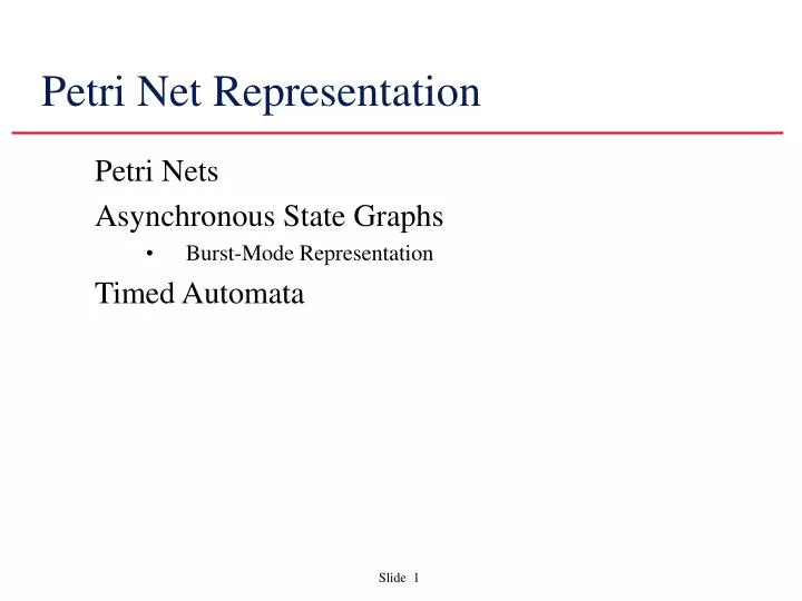
Petri Net Representation. Petri Nets Asynchronous State Graphs Burst-Mode Representation Timed Automata. Petri Nets. Reference: Tadao Murata. “ Petri nets: Properties, Analysis and Applications. ” Proc. of the IEEE, 77(4), 1989. available on class website.

E N D
Petri Net Representation • Petri Nets • Asynchronous State Graphs • Burst-Mode Representation • Timed Automata
Petri Nets • Reference: • Tadao Murata. “Petri nets: Properties, Analysis and Applications.” Proc. of the IEEE, 77(4), 1989. • available on class website
Petri Nets: Properties, Analysis and Applications Based on paper by T. Murata
Outline • Introduction/History • Transition enabling & firing • Modeling examples • Behavioral properties • Analysis methods • Liveness, safeness & reachability • Analysis & synthesis of Marked Graphs • Structural properties • Modified Petri Nets
Introduction • Petri Nets • concurrent, asynchronous, distributed, parallel, nondeterministic and/or stochastic systems • graphical tool • visual communication aid • mathematical tool • state equations, algebraic equations, etc • communication between theoreticians and practitioners
History • 1962: C.A. Petri’s dissertation (U. Darmstadt, W. Germany) • 1970: Project MAC Conf. on Concurrent Systems and Parallel Computation (MIT, USA) • 1975: Conf. on Petri Nets and related Methods (MIT, USA) • 1979: Course on General Net Theory of Processes and Systems (Hamburg, W. Germany) • 1980: First European Workshop on Applications and Theory of Petri Nets (Strasbourg, France) • 1985: First International Workshop on Timed Petri Nets (Torino, Italy)
Applications • performance evaluation • communication protocols • distributed-software systems • distributed-database systems • concurrent and parallel programs • industrial control systems • discrete-events systems • multiprocessor memory systems • dataflow-computing systems • fault-tolerant systems • etc, etc, etc
Definition • Directed, weighted, bipartite graph • places • transitions • arcs (places to transitions or transitions to places) • weights associated with each arc • Initial marking • assigns a non-negative integer to each place
Transition (firing) rule • A transition t is enabled if each input place p has at least w(p,t) tokens • An enabled transition may or may not fire • A firing on an enabled transition t removes w(p,t) from each input place p, and adds w(t,p’) to each output place p’
Firing example • 2H2 + O2 2H2O 2 t H2 2 H2O O2
Firing example • 2H2 + O2 2H2O 2 t H2 2 H2O O2
Some definitions • source transition: no inputs • sink transition: no outputs • self-loop: a pair (p,t) s.t. p is both an input and an output of t • pure PN: no self-loops • ordinary PN: all arc weights are 1’s • infinite capacity net: places can accommodate an unlimited number of tokens • finite capacity net: each place p has a maximum capacity K(p) • strict transition rule: after firing, each output place can’t have more than K(p) tokens • Theorem: every pure finite-capacity net can be transformed into an equivalent infinite-capacity net
Modeling FSMs vend 15¢ candy 10 15 5 5 5 5 0 5 10 10 20 10 vend 20¢ candy
Modeling FSMs vend 15¢ candy 10 5 state machines: each transition has exactly one input and one output 5 5 5 10 10 vend 20¢ candy
Modeling FSMs vend 10 5 conflict, decision or choice 5 5 5 10 10 vend
Modeling concurrency t2 marked graph: each place has exactly one incoming arc and one outgoing arc. t1 t4 t3
Modeling concurrency concurrency t2 t1 t4 t3
Modeling dataflow computation • x = (a+b)/(a-b) a copy + / x a+b a !=0 b copy - a-b NaN b =0
Modeling communication protocols ready to send ready to receive buffer full send msg. receive msg. wait for ack. proc.2 proc.1 msg. received receive ack. send ack. buffer full ack. received ack. sent
Modeling synchronization control k k writing k reading k
Behavioral properties (1) • Properties that depend on the initial marking • Reachability • Mn is reachable from M0 if exists a sequence of firings that transform M0 into Mn • reachability is decidable, but exponential • Boundedness • a PN is bounded if the number of tokens in each place doesn’t exceed a finite number k for any marking reachable from M0 • a PN is safe if it is 1-bounded
Behavioral properties (2) • Liveness • a PN is live if, no matter what marking has been reached, it is possible to fire any transition with an appropriate firing sequence • equivalent to deadlock-free • strong property, different levels of liveness are defined (L0=dead, L1, L2, L3 and L4=live) • Reversibility • a PN is reversible if, for each marking M reachable from M0, M0 is reachable from M • relaxed condition: a marking M’ is a home state if, for each marking M reachable from M0, M’ is reachable from M
Behavioral properties (3) • Coverability • a marking is coverable if exists M’ reachable from M0 s.t. M’(p)>=M(p) for all places p • Persistence • a PN is persistent if, for any two enabled transitions, the firing of one of them will not disable the other • then, once a transition is enabled, it remains enabled until it’s fired • all marked graphs are persistent • a safe persistent PN can be transformed into a marked graph
Analysis methods (1) • Coverability tree • tree representation of all possible markings • root = M0 • nodes = markings reachable from M0 • arcs = transition firings • if net is unbounded, then tree is kept finite by introducing the symbol • Properties • a PN is bounded iff doesn’t appear in any node • a PN is safe iff only 0’s and 1’s appear in nodes • a transition is dead iff it doesn’t appear in any arc • if M is reachable form M0, then exists a node M’ that covers M
Coverability tree example M0=(100) p1 t3 p2 t1 t0 t2 p3
Coverability tree example M0=(100) t1 p1 t3 M1=(001) “dead end” p2 t1 t0 t2 p3
Coverability tree example M0=(100) t1 t3 p1 t3 M1=(001) “dead end” M3=(10) p2 t1 t0 t2 p3
Coverability tree example M0=(100) t1 t3 p1 t3 M1=(001) “dead end” M3=(10) t1 p2 t1 t0 M4=(01) t2 p3
Coverability tree example M0=(100) t1 t3 p1 t3 M1=(001) “dead end” M3=(10) t1 t3 p2 t1 t0 M4=(01) M3=(10) “old” t2 p3
Coverability tree example M0=(100) t1 t3 p1 t3 M1=(001) “dead end” M3=(10) t1 t3 p2 t1 t0 M4=(01) M6=(10) “old” t2 t2 p3 M5=(01) “old”
Coverability tree example M0=(100) 100 t1 t3 t1 t3 M1=(001) “dead end” M3=(10) 001 10 t1 t3 t1 t3 M4=(01) M6=(10) “old” 01 t2 t2 M5=(01) “old” coverability graph coverability tree
Subclasses of Petri Nets (1) • Ordinary PNs • all arc weights are 1’s • same modeling power as general PN, more convenient for analysis but less efficient • State machine • each transition has exactly one input place and exactly one output place • Marked graph • each place has exactly one input transition and exactly one output transition
Subclasses of Petri Nets (2) • Free-choice • every outgoing arc from a place is either unique or is a unique incoming arc to a transition • Extended free-choice • if two places have some common output transition, then they have all their output transitions in common • Asymmetric choice (or simple) • if two places have some common output transition, then one of them has all the output transitions of the other (and possibly more)
Subclasses of Petri Nets (3) PN PN AC EFC FC SM MG
Liveness and Safeness Criteria (1) • general PN • if a PN is live and safe, then there are no source or sink places and source or sink transitions • if a connected PN is live and safe, then the net is strongly connected • SM • a SM is live iff the net is strongly connected and M0 has at least one token • a SM is safe iff M0 has at most one token
Liveness and Safeness Criteria (2) • MG • a MG is equivalent to a marked directed graph (arcs=places, nodes=transitions) • a MG is live iff M0 places at least one token on each directed circuit in the marked directed graph • a live MG is safe iff every place belongs to a directed circuit on which M0 places exactly one token • there exists a live and safe marking in a directed graph iff it is strongly connected