Download
1 / 24
240 likes | 340 Views
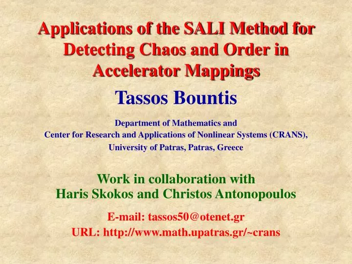
Applications of the SALI Method for Detecting Chaos and Order in Accelerator Mappings. Tassos Bountis Department of Mathematics and Center for Research and Applications of Nonlinear Systems (CRANS), University of Patras, Patras, Greece Work in collaboration with

E N D
Applications of the SALI Method for Detecting Chaos and Order in Accelerator Mappings Tassos Bountis Department of Mathematics and Center for Research and Applicationsof Nonlinear Systems (CRANS), University of Patras, Patras, Greece Work in collaboration with Haris Skokos and Christos Antonopoulos E-mail: tassos50@otenet.gr URL: http://www.math.upatras.gr/~crans
Outline • Definition of the SALI Criterion • Behavior of the SALI Criterion • Ordered orbits • Chaotic orbits • Applications to: • 2D maps • 4D maps • 2D Hamiltonians (Hénon-Heiles system) • 3D Hamiltonians • 4D maps of accelerator dynamics • Conclusions
Definition of the Smaller Alignment Index (SALI) Consider the k-dimensional phase space of a conservative dynamical system(e.g. a Hamiltonian flow or a symplectic map), which may be continuous in time (k =2N) or discrete: (k=2M). Suppose we wish to study the behavior of an orbit in that space X(t), or X(n), with initial condition : X(0)=(x1(0), x2(0),…,xk(0))
Consider a nearby orbit X’ with deviation vectorV(t), or V(n), and initial condition V(0) =X’(0) – X(0) =(Δx1(0), Δx2 (0),…, Δxk(0)) To study the dynamics of X(t) - or X(n) – one usually follows the evolution of onedeviation vectorV(t) or V(n), by solving: • Either the linear (variational)ODEs (for flows) • Or the linearized (tangent) map (for discrete dynamics) where DF is the Jacobian matrix evaluated at the points of the orbit under study.
Two different behaviors are distinguished: • The two vectors V1 , V2 tend to coincide or become opposite along the most unstable direction • SALI(t) →0and theorbit X(t) is chaotic • There is no unstable direction, the deviation vectors tend to become tangent to a torus and • SALI(t) ~ constantandthe orbit X(t) is regular We shall follow the evolution in time of two different initial deviation vectors (e.g. V1(0), V2(0)), and define SALI (Skokos Ch., 2001, J. Phys. A, 34, 10029) as:
Choosing 2 vectorsalong the 2 independent directions: • fH=( Hpx, Hpy, -Hx, -Hy), fF=( Fpx, Fpy, -Fx, -Fy) • and 2 vectors perpendicular to these directions: • H=(Hx, Hy, Hpx, Hpy), F=(Fx, Fy, Fpx, Fpy) Behavior of SALIfor ordered motion (Skokos & Bountis, 2003, Prog. Th. Phys. Supp., 150, 439) Suppose we have an integrable 2D Hamiltonian system with integrals H and F. Form avector basis of the 4D phase space: A general deviation vector can then be written as a linear combination:
We have found thatall deviation vectors, V(t), tend to the tangent space of the torus, since a1,a2 oscillate, while |a3|, |a4| ~ t-1→0 as t→∞. as, for example, in the Hamiltonian: which for B=3A and any E has a second integral:F=(xpy– y px)2
Behavior of the SALI for chaotic motion (Skokos and Bountis, 2004, J. Phys. A, 37, 6269) +… The evolution of a deviation vector can be approximated by : where σ1>σ2>… are the Lyapunov exponents. Thus, we derive a leading order estimate for v1(t) : and an analogous expression for v2(t): So we get:
We have tested the validity of this important approximation SALI ~ exp[-(σ1-σ2)t] on many examples, like the 3D Hamiltonian: with ω1=1, ω2=1.4142, ω3=1.7321, Η=0.09 σ1=0.037=Lmax Slope= –(σ1-σ2) σ2=0.011
Applications – 2D map For ν=0.5 we consider the orbits: ordered orbit A with initial conditions x1=2, x2=0. chaotic orbit B with initial conditions x1=3, x2=0.
Applications – 4D map For ν=0.5, κ=0.1, μ=0.1 we consider the orbits: ordered orbit C with initial conditions x1=0.5, x2=0, x3=0.5, x4=0. chaotic orbit D with initial conditions x1=3, x2=0, x3=0.5, x4=0. C D D C After N~8000 iterations SALI~10-8
Applications – Hénon-Heiles system For E=1/8 we consider the orbits with initial conditions: Ordered orbit, x=0, y=0.55, px=0.2417, py=0 Chaotic orbit, x=0, y=-0.016, px=0.49974, py=0 Chaotic orbit, x=0, y=-0.01344, px=0.49982, py=0
t=1000 t=4000 Applications – Hénon-Heiles system Initial conditions taken on the y – axis (x=0, py=0)
E=1/8 t=1000 py y Applications – Hénon-Heiles system
Behavior of the SALI for ordered and chaotic orbits Color plot of the subspace x, px with initial conditions y=z=py=0, pz>0 Applications – 3D Hamiltonian We consider the 3D Hamiltonian with A=0.9, B=0.4, C=0.225, ε=0.56, η=0.2, H=0.00765.
Applications – 4D Accelerator map We consider the 4D symplectic map describing the instantaneous “kicks” experienced by a proton beam as it passes through magnetic focusing elements of the FODO cell type (see Turchetti & Scandale 1991, Vrahatis & Bountis, IJBC, 1996, 1997). Here x1 and x3 are the particle’s horizontal and vertical deflections from the ideal circular orbit, x2 and x4 are the associated momenta and ω1, ω2are related to the accelerator’s tunes qx , qy by ω1=2πqx, ω2=2πqy Our problem is to estimate the region of stability of the particle’s motion (the so-called dynamical aperture of the beam)
In Vrahatis and Bountis, IJBC, 1996, 1997, we computed near the boundary of escapestable periodic orbits of very long period, e.g. 13237 (!). Note that SALI convergeslong before Lmax becomes zero. qx =0.61903 qy =0.4152
Making a small perturbation in the x - tune Δqx =-0.001, i.e. with qx =0.61803 qy =0.4152, we detect ordered motion near an 8 – tori resonance
points with |x3|<0.04 SALI quickly detects the thin chaotic layer around the 8-tori resonance
Near the beam’s dynamical aperture, SALI quickly detects a chaotic orbit, which eventually escapes after about 82000 iterations (qx=0.628615 qy=0.4152)
A more “global” study of the dynamics: • We compute orbits with x1 varying from 0 to 0.9, while x2, x3, x4 are the same as in the orbit of the 8-tori resonancePlotting SALI after N=105 iterations for each point on this line we find:
2. We consider 1,922,833 orbits by varying all x1, x2, x3, x4 within spherical shells of width 0.01 in a hypersphere of radius 1. (qx=0.61803 qy=0.4152)
Conclusions • The Small Alignment Index (SALI) is an efficient criterion for distiguishing ordered from chaotic motion in Hamiltonian flows and symplectic maps of any dimensionality. • It has significant advantages over the usual computation of Lyapunov exponents. • It can be used to characterize individual orbits as well as “chart” chaotic and regular domains of different scales and sizes in phase space. • It has been successfully applied to “trace out” the dynamical aperture of proton beamsin 2 space dimensions, passing repeatedly through FODO cell magnetic focusing elements. • We are now generalizing our results by adding to our models space charge effects and synchrotron oscillations.
References • Vrahatis M., Bountis, T. et al. (1996) IJBC, vol. 6 (8), 1425. • Vrahatis M., Bountis, T. et al. (1997), IJBC, vol. 7 (12), 2707. • Skokos Ch. (2001) J. Phys. A, 34, 10029. • Skokos Ch., Antonopoulos Ch., Bountis T. C. & Vrahatis M. (2003) Prog. Theor. Phys. Supp., 150, 439. • Skokos Ch., Antonopoulos Ch., Bountis T. C. & Vrahatis M. (2004) J. Phys. A, 37, 6269.