Download
1 / 90
900 likes | 1.09k Views
ENEE699/ENEE459P: Parallel Algorithms Home page: http://www.umiacs.umd.edu/users/vishkin/TEACHING/enee459p-f10.html. Uzi Vishkin Electrical and Computer Engineering Dept. Topics covered. Parallel algorithms Parallel programing languages

E N D
ENEE699/ENEE459P: Parallel AlgorithmsHome page:http://www.umiacs.umd.edu/users/vishkin/TEACHING/enee459p-f10.html Uzi Vishkin Electrical and Computer Engineering Dept
Topics covered • Parallel algorithms • Parallel programing languages • Very limited: Parallel programming techniques focusing on tuning programs for performance. • The course will build on your knowledge of algorithms, data structures, and programming.
Why? • Yesterday: Top of the line machines were parallel • Today: Parallelism is the norm for all classes of machines, from mobile devices to the fastest machines.
An experimental course • The course will be a bit unique • We want to learn about teaching strategies to improve the course • For a month (tentatively: September 8-October 6) The course will join a similar course from the University of Illinois via teleconference • The professor from Illinois will teach a simple programming model (OpenMP) and I will teach a different model (and follow a different style) • Programming assignment 1 and 2 will be two parallel programs each. By doing them you will learn about two different parallel programming models and will be able to compare the difficulty of each model [Note At Illinois programming assignments are called machine problems (MPs)] • This is in itself an interesting learning experience • We will ask for your help to gather data, but contributing the data will be completely voluntary (and I will not know if you are contributing the data until the course is over and grades have been assigned). If you choose to participate in the evaluation, you will tell us how many hours it took you to complete each assignment. This information, in combination with the quality of the program you produce, will tell us about the effectiveness of learning of each model • We will also learn about jointly teaching across universities
Course organization Official course website: http://www.umiacs.umd.edu/users/vishkin/TEACHING/enee459p-f10.html FYI only: The website for the Illinois course is https://agora.cs.illinois.edu/display/cs420fa10/Home Grading (slightly revised to reflect update in joint plans with U. Illinois): • 10% - Written homework • 40% - Programming projects • 20% - Mid-term exam, October 11, in class • 30% - Final exam (comprehensive), 8:00-10:00 Saturday, December 18 (based on Testudo)
Tentative Schedule, till Oct 11 midterm • Introduction and brief review of shared-memory machines towards joint sessions (8/30,9/1) Joint sessions • Shared-memory programming in OpenMP (9/8,9/13) • Parallel algorithms and programming projects in XMT-C and OpenMP (9/15-10/6)
Commodity computer systems Chapter 1 19462003:Serial. 5KHz4GHz. Chapter 2 2004--: Parallel. #”cores”:~dy-2005 2005: 1 core. 2015: 100 (?) cores 2020: 1000 (?) cores Windows 7: scales to 256 cores… how to use the remaining 255? Is this the role of the OS? BIG NEWS Clock frequency growth: flat. If you want your program to run significantly faster … you’re going to have to parallelize it Parallelism: only game in town #Transistors/chip 19802010s: 29K30B! Programmer’s IQ? Flat.. 40 years of parallel computing The world is yet to see a successful general-purpose parallel computer: Easy to program & good speedups Intel Platform 2015, March05
The Pain of Parallel Programming Parallel programming is currently too difficult: To many users programming existing parallel computers is “as intimidating and time consuming as programming in assembly language” [NSF Blue-Ribbon Panel on Cyberinfrastructure]. AMD/Intel: “Need PhD in CS to program today’s multicores”. 40yr old problem: Parallel architectures built using the following “methodology”: build-first figure-out-how-to-program-later. [J. Hennessy: “Many of the early ideas were motivated by observations of what was easy to implement in the hardware rather than what was easy to use”] Tribal lore, parallel programming profs, DARPA HPCS Development Time study (2004-2008): “Parallel algorithms and programming for parallelism is easy. What is difficult is the programming/tuningfor performance that comes after that.” Current course & Illinois learnability experiment, 1st revisit: How to best learn the material?
Welcome to the 2010 Impasse All vendors committed to multi-cores. Yet, their architecture not stable; The Trouble with Multicore: Chipmakers are busy designing microprocessors that most programmers can't handle—D. Patterson, IEEE Spectrum Jul’10. The software spiral (HW improvements SW imp HW imp) – growth engine for IT (A. Grove, Intel); Alas, now broken! SW vendors avoid investment in long-term SW development since may bet on the wrong horse. Impasse bad for business. Parallel programming education: Does CS&E degree mean: being trained for a 50yr career dominated by parallelism by programming yesterday’s serial computers? If no, why not same impasse? My original position, 2nd visit of course objectives: Can teach common denominator (grad, seniors, freshmen, HS) State-of-the-art: only the education enterprise has an actionable agenda! tie-breaker!
2 Paradigm Shifts • Serial to parallel: widely agreed • Within parallel: Existing “decomposition-first” paradigm. Painful to program. Proposed paradigm. Express only “what can be done in parallel”. Easy-to-program.
Abstractions in CS • Any particular word of an indefinitely large memory is immediately available • A uniprocessor is serving the task that the user is currently working on exclusively. (i) abstracts away a hierarchy of memories, each has greater capacity, but slower access time, than the preceding one. (ii) abstracts way: virtual file systems that can be implemented in local storage or a local or global network, the (whole) web, and other tasks that may be concurrently using the same computer system. These abstractions have improved productivity of programmers and other users, and contributed towards broadening participation in computing. • The proposed addition to this consensus is as follows. That an indefinitely large number of operations available for concurrent execution executes immediately.
But, what is this common denominator? Serial RAM Step: 1 op (memory/etc), unit time PRAM, Parallel Random-Access Model Step: many ops, unit time Serial doctrine Natural (parallel) algorithm time = #ops time << #ops How to tell this to children? In the beginning: no internet. Not even computers. Then, CS was created in just two days: 1st day: mathematical induction [ same] 2nd day: ‘each op’ in unit time [ ‘any number of concurrent ops’ in unit time] Chronology of approach 1979- : THEORY figure out how to think algorithmically in parallel 1997- : PRAM-On-Chip@UMD: derive specs for architecture; design and build Note 2 issues: (i) parallel algorithmic thinking, (ii) specs first. What could I do in parallel at each step assuming unlimited hardware . . # ops . . # ops . . .. .. .. .. time time
Flavor of parallelism Exchange Problem Replace A and B. Ex. A=2,B=5A=5,B=2. Serial Alg: X:=A;A:=B;B:=X. 3 Ops. 3 Steps. Space 1. Fewer steps (FS): X:=A B:=X Y:=B A:=Y 4 ops. 2 Steps. Space 2. Array Exchange Problem Given A[1..n] & B[1..n], replace A(i) and B(i), i=1..n. Serial Alg: For i=1 to n do X:=A(i);A(i):=B(i);B(i):=X /*serial replace 3n Ops. 3n Steps. Space 1. Par Alg1: For i=1 to n pardo X(i):=A(i);A(i):=B(i);B(i):=X(i) /*serial replace in parallel 3n Ops. 3 Steps. Space n. Par Alg2: For i=1 to n pardo X(i):=A(i) B(i):=X(i) Y(i):=B(i) A(i):=Y(i) /*FS in parallel 4n Ops. 2 Steps. Space 2n. Discussion Parallelism requires extra space (memory). Par Alg 1 clearly faster than Serial Alg. Is Par Alg 2 preferred to Par Alg 1?
Snapshot: XMT High-level language XMTC: Single-program multiple-data (SPMD) extension of standard C. Includes Spawn and PS - a multi-operand instruction. Short (not OS) threads. Cartoon Spawn creates threads; a thread progresses at its own speed and expires at its Join. Synchronization: only at the Joins. So, virtual threads avoid busy-waits by expiring. New: Independence of order semantics (IOS). Array Exchange. Pseudo-code for Par Alg1 Spawn(1,n){ X($):=A($);A($):=B($);B($):=X($) }
Input: (i) All world airports. (ii) For each, all airports to which there is a non-stop flight. Find: smallest number of flights from DCA to every other airport. Basic algorithm Step i: For all airports requiring i-1flights For all its outgoing flights Mark (concurrently!) all “yet unvisited” airports as requiring i flights (note nesting) Serial: uses “serial queue”. O(T) time; T – total # of flights Parallel: parallel data-structures. Inherent serialization: S. Gain relative to serial: (first cut) ~T/S! Decisive also relative to coarse-grained parallelism. Note: (i) “Concurrently”: only change to serial algorithm (ii) No “decomposition”/”partition” KEY POINT: Mental effort of PRAM-like programming is considerably easier than for any of the computers currently sold. Understanding falls within the common denominator of other approaches. Example of PRAM-like Algorithm
Back to the education crisis CTO of NVidia and the official Intel leader of multi-cores at Intel: teach parallelism as early as you. Reason: we don’t only under teach. We misteach, since students acquire bad habits. Converged to: Teach CS&E Freshmen and invite all Eng, Math, and Science; sends message “CS&E is where the action is”. Why should you care? Programmability is a necessary condition for success of a many core platform. Teachability is necessary for that and is a practical benchmark.
A case for XMT in current study Recall how the standard CS curriculum looks: 1st year of CS: programming. Later: design & analysis of algorithms. Rationale: 1st concrete programming experience, so that algorithms & analysis make sense But, you can understand parallel algorithm, which is an academic-credit-worthy topic (beyond 1st year), learn skill of parallel programming, by assignments on par with Parallel Prog courses. And you do not need to know anything about parallel architectures. In fact, the review of shared memory architecture deviates from my normal way of presenting parallel algorithms and XMT programming. Architecture is noted in the last class only.
Need A general-purpose parallel computer framework [“successor to the Pentium for the multi-core era”] that: is easy to program; gives good performance with any amount of parallelism provided by the algorithm; namely, up- and down-scalability including backwards compatibility on serial code; supports application programming (VHDL/Verilog, OpenGL, MATLAB) and performance programming; and fits current chip technology and scales with it. (in particular: strong speed-ups for single-task completion time) Main Point of talk: PRAM-On-Chip@UMD is addressing (i)-(iv).
Summary of technical pathwaysIt is all about (2nd class) levers Credit: Archimedes • Parallel algorithms. First principles. Alien culture: had to do from scratch. (No lever) • Levers: • 1. Input: Parallel algorithm. Output: Parallel architecture. • 2. Input: Parallel algorithms & architectures. Output: parallel programming
The PRAM Rollercoaster ride Late 1970’s Theory work began UP Won the battle of ideas on parallel algorithmic thinking. No silver or bronze! Model of choice in all theory/algorithms communities. 1988-90: Big chapters in standard algorithms textbooks. DOWN FCRC’93: “PRAM is not feasible”. [‘93+ despair no good alternative! Where vendors expect good enough alternatives to come from in 2010?]; Device changed it all: UP Highlights: eXplicit-multi-threaded (XMT) FPGA-prototype computer (not simulator), SPAA’07,CF’08; 90nm ASIC tape-outs: int. network, HotI’07, XMT. # on-chip transistors How come? crash “course” on parallel computing How much processors-to-memories bandwidth? Enough: Ideal Programming Model (PRAM) Limited: Programming difficulties
PRAM-On-Chip Reduce general-purpose single-task completion time. Go after any amount/grain/regularity of parallelism you can find. Premises (1997): within a decade transistor count will allow an on-chip parallel computer (1980: 10Ks; 2010: 10Bs) Will be possible to get good performance out of PRAM algorithms Speed-of-light collides with 20+GHz serial processor. [Then came power ..] Envisioned general-purpose chip parallel computer succeeding serial by 2010 Processors-to-memories bandwidth: One of several basic differences relative to “PRAM realization comrades”: NYU Ultracomputer, IBM RP3, SB-PRAM and MTA. PRAM was just ahead of its time. Not many examples in the computer area where patience is a virtue. Culler-Singh 1999: “Breakthrough can come from architecture if we can somehow…truly design a machine that can look to the programmer like a PRAM”.
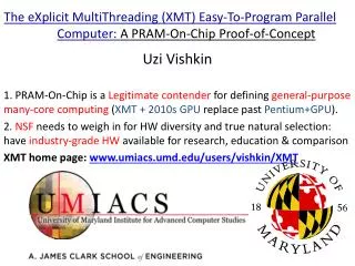
The eXplicit MultiThreading (XMT) Easy-To-Program Parallel Computer www.umiacs.umd.edu/users/vishkin/XMT
The XMT Overall Design Challenge Assume algorithm scalability is available. Hardware scalability: put more of the same ... but, how to manage parallelism coming from a programmable API? Spectrum of Explicit Multi-Threading (XMT) Framework Algorithms −− > architecture −− > implementation. XMT: strategic design point for fine-grained parallelism New elements are added only where needed Attributes Holistic: A variety of subtle problems across different domains must be addressed: Understand and address each at its correct level of abstraction
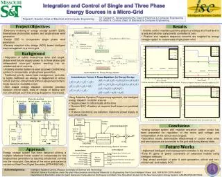
64-processor, 75MHz prototype Notes: 80% of FPGA C was used. BRAM: FPGA-built-in SRAM.
Naming Contest for New Computer Paraleap chosen out of ~6000 submissions Single (hard working) person (X. Wen) completed synthesizable Verilog description AND the new FPGA-based XMT computer in slightly more than two years. No prior design experience. Attests to: basic simplicity of the XMT architecture faster time to market, lower implementation cost.
Experience with new FPGA computer Included: basic compiler [Tzannes,Caragea,Barua,V]. New computer used: to validate past speedup results. Spring’07 parallel algorithms graduate class @UMD - Standard PRAM class. 30 minute review of XMT-C. - Reviewed the architecture only in the last week. - 6(!) significant programming projects (in a theory course). - FPGA+compiler operated nearly flawlessly. Sample speedups over best serial by students Selection: 13X. Sample sort: 10X. BFS: 23X. Connected components: 9X. Students’ feedback: “XMT programming is easy” (many), “The XMT computer made the class the gem that it is”, “I am excited about one day having an XMT myself! ” 11-12,000X relative to cycle-accurate simulator in S’06. Over an hour sub-second. (Year46 minutes.)
Experience with High School Students, Fall’07 1-day parallel algorithms tutorial to 12 HS students. Some (2 10th graders) managed 8 programming assignments, including 5 of the 6 in the grad course. Only help: 1 office hour/week by undergrad TA. No school credit. Part of a computer club after 8 periods/day. One of these 10th graders: “I tried to work on parallel machines at school, but it was no fun: I had to program around their engineering. With XMT, I could focus on solving the problem that I had to solve.” Dec’08-Jan’09: 50 HS students, by self-taught HS teacher, TJ HS, Alexandria, VA. Part of the regular curriculum. By summer’09: 100+ K-12 students have experienced XMT. ‘09 MCPS Middle school camp for children from underepresented groups. Taught at Baltimore Poly HS: 70% African Americans. Spring’09: Course to Freshmen, UMD (strong enrollment). How will programmers have to think by the time you graduate. SIGCSE’10 paper and CS4HS’09@CMU Keynote
NEW: Software release Allows to use your own computer for programming on an XMT environment and experimenting with it, including: Cycle-accurate simulator of the XMT machine Compiler from XMTC to that machine Also provided, extensive material for teaching or self-studying parallelism, including Tutorial + manual for XMTC (150 pages) Classnotes on parallel algorithms (100 pages) Video recording of 9/15/07 HS tutorial (300 minutes) Video recording of Spring’09 grad course (30+ hours) Next Major Objective Industry-grade chip and production quality compiler. Requires 10X in funding.
Participants Grad students:, Aydin Balkan, PhD, George Caragea, James Edwards, David Ellison, Mike Horak, MS, Fuat Keceli, Beliz Saybasili, Alex Tzannes, Xingzhi Wen, PhD Industry design experts (pro-bono). Rajeev Barua, Compiler. Co-advisor of 2 CS grad students. 2008 NSF grant. Gang Qu, VLSI and Power. Co-advisor. Steve Nowick, Columbia U., Asynch computing. Co-advisor. 2008 NSF team grant. Ron Tzur, Purdue U., K12 Education. Co-advisor. 2008 NSF seed funding K12:Montgomery Blair Magnet HS, MD, Thomas Jefferson HS, VA, Baltimore (inner city) Ingenuity Project Middle School 2009 Summer Camp, Montgomery County Public Schools Marc Olano, UMBC, Computer graphics. Co-advisor. Tali Moreshet, Swarthmore College, Power. Co-advisor. Marty Peckerar, Microelectronics Igor Smolyaninov, Electro-optics Funding: NSF, NSA 2008 deployed XMT computer, NIH Industry partner: Intel Reinvention of Computing for Parallelism. Selected for Maryland Research Center of Excellence (MRCE) by USM, 12/08. Not yet funded. 17 members, including UMBC, UMBI, UMSOM. Mostly applications.
Parallel Random-Access Machine/Model PRAM: • n synchronous processors all having unit time access to a shared memory. • Each processor has also a local memory. • At each time unit, a processor can: • write into the shared memory (i.e., copy one of its local memory registers into • a shared memory cell), • 2. read into shared memory (i.e., copy a shared memory cell into one of its local • memory registers ), or • 3. do some computation with respect to its local memory.
pardo programming construct - for Pi , 1 ≤ i ≤ n pardo - A(i) := B(i) This means The following n operations are performed concurrently: processor P1 assigns B(1) into A(1), processor P2 assigns B(2) into A(2), …. Modeling read&write conflicts to the same shared memory location Most common are: - exclusive-read exclusive-write (EREW) PRAM: no simultaneous access by more than one processor to the same memory location for read or write purposes • concurrent-read exclusive-write (CREW) PRAM: concurrent access for reads but not for writes • concurrent-read concurrent-write (CRCW allows concurrent access for both reads and writes. We shall assume that in a concurrent-write model, an arbitrary processor among the processors attempting to write into a common memory location, succeeds. This is called the Arbitrary CRCW rule. There are two alternative CRCW rules: (i) Priority CRCW: the smallest numbered, among the processors attempting to write into a common memory location, actually succeeds. (ii) Common CRCW: allows concurrent writes only when all the processors attempting to write into a common memory location are trying to write the same value.
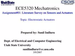
Example of a PRAM algorithm: The summation problem Input An array A = A(1) . . .A(n) of n numbers. The problem is to compute A(1) + . . . + A(n). The summation algorithm works in rounds. Each round: add, in parallel, pairs of elements: add each odd-numbered element and its successive even-numbered element. If n = 8, outcome of 1st round is: A(1) + A(2), A(3) + A(4), A(5) + A(6), A(7) + A(8) Outcome of 2nd round: A(1) + A(2) + A(3) + A(4), A(5) + A(6) + A(7) + A(8) and the outcome of 3rd (and last) round: A(1) + A(2) + A(3) + A(4) + A(5) + A(6) + A(7) + A(8) B – 2-dimensional array (whose entries are B(h,i), 0 ≤ h ≤ log n and 1 ≤ i ≤ n/2h) used to store all intermediate steps of the computation (base of logarithm: 2). For simplicity, assume n = 2k for some integer k. ALGORITHM 1 (Summation) 1. for Pi , 1 ≤ i ≤ n pardo 2. B(0, i) := A(i) 3. for h := 1 to log n do 4. if i ≤ n/2h 5. then B(h, i) := B(h − 1, 2i − 1) + B(h − 1, 2i) 6. else stay idle 7. for i = 1: output B(log n, 1); for i > 1: stay idle Algorithm 1 uses p = n processors. Line 2 takes one round, Line 3 defines a loop taking log n rounds Line 7 takes one round.
Summation on an n = 8 processor PRAM Again Algorithm 1 uses p = n processors. Line 2 takes one round, line 3 defines a loop taking log n rounds, and line 7 takes one round. Since each round takes constant time, Algorithm 1 runs in O(log n) time. [When you see O (“big Oh”), think “proportional to”.] So, an algorithm in the PRAM model is presented in terms of a sequence of parallel time units (or “rounds”, or “pulses”); we allow p instructions to be performed at each time unit, one per processor; this means that a time unit consists of a sequence of exactly p instructions to be performed concurrently. So, an algorithm in the PRAM model is presented in terms of a sequence of parallel time units (or “rounds”, or “pulses”); we allow p instructions to be performed at each time unit, one per processor; this means that a time unit consists of a sequence of exactly p instructions to be performed concurrently.
2 drawbacks to PRAM mode: (i) Does not reveal how the algorithm will run on PRAMs with different number of processors; e.g., to what extent will more processors speed the computation, or fewer processors slow it? (ii) Fully specifying the allocation of instructions to processors requires a level of detail which might be unnecessary (a compiler may be able to extract from lesser detail) Work-Depth presentation of algorithms Alternative model and presentation mode. Work-Depth algorithms are also presented as a sequence of parallel time units (or “rounds”, or “pulses”); however, each time unit consists of a sequence of instructions to be performed concurrently; the sequence of instructions may include any number.
WD presentation of the summation example “Greedy-parallelism”: At each point in time, the (WD) summation algorithm seeks to break the problem into as many pair wise additions as possible, or, in other words, into the largest possible number of independent tasks that can performed concurrently. ALGORITHM 2 (WD-Summation) 1. for i , 1 ≤ i ≤ n pardo 2. B(0, i) := A(i) 3. for h := 1 to log n 4. for i , 1 ≤ i ≤ n/2h pardo 5. B(h, i) := B(h − 1, 2i − 1) + B(h − 1, 2i) 6. for i = 1 pardo output B(log n, 1) The 1st round of the algorithm (lines 1&2) has n operations. The 2nd round (lines 4&5 for h = 1) has n/2 operations. The 3rd round (lines 4&5 for h = 2) has n/4 operations. In general, the k-th round of the algorithm, 1 ≤ k ≤ log n + 1, has n/2k-1 operations and round log n +2 (line 6) has one more operation (use of a pardo instruction in line 6 is somewhat artificial). The total number of operations is 2n and the time is log n + 2. We will use this information in the corollary below. The next theorem demonstrates that the WD presentation mode does not suffer from the same drawbacks as the standard PRAM mode, and that every algorithm in the WD mode can be automatically translated into a PRAM algorithm.
The WD-presentation sufficiency Theorem Consider an algorithm in the WD mode that takes a total of x = x(n) elementary operations and d = d(n) time. The algorithm can be implemented by any p = p(n)-processor PRAM within O(x/p + d) time, using the same concurrent-write convention as in the WD presentation. [i.e., 5 theorems: EREW, CREW, Common/Arbitrary/Priority CRCW] Proof xi - # instructions at round i. [x1+x2+..+xd = x] p processors can simulate xiinstructions in ⌈xi/p⌉≤ xi/p + 1 time units. See next slide. Demonstration in Algorithm 2’ shows why you don’t want to leave this to a programmer. Formally: first reads, then writes. Theorem follows, since ⌈x1/p⌉+⌈x2/p⌉+..+⌈xd/p⌉≤ (x1/p +1)+..+(xd/p +1) ≤ x/p + d
Round-robin emulation of y concurrent instructions by p processors in ⌈y/p⌉ rounds. In each of the first ⌈y/p⌉ −1 rounds, p instructions are emulated for a total of z = p(⌈y/p⌉ − 1) instructions. In round ⌈y/p⌉, the remaining y − z instructions are emulated, each by a processor, while the remaining w − y processor stay idle, where w = p⌈y/p⌉
Corollary for summation example Algorithm 2 would run in O(n/p + log n) time on a p-processor PRAM. For p ≤ n/ log n, this implies O(n/p) time. Later called both optimal speedup & linear speedup For p ≥ n/ log n: O(log n) time. Since no concurrent reads or writes p-processor EREW PRAM algorithm.
ALGORITHM 2’ (Summation on a p-processor PRAM) 1. for Pi , 1 ≤ i ≤ p pardo 2. for j := 1 to ⌈n/p⌉ − 1 do - B(0, i + (j − 1)p) := A(i + (j − 1)p) 3. for i , 1 ≤ i ≤ n − (⌈n/p⌉ − 1)p - B(0, i + (⌈n/p⌉ − 1)p) := A(i + (⌈n/p⌉ − 1)p) - for i , n − (⌈n/p⌉ − 1)p ≤ i ≤ p - stay idle 4. for h := 1 to log n 5. for j := 1 to ⌈n/(2hp)⌉ − 1 do (*an instruction j := 1 to 0 do means: - “do nothing”*) • B(h, i+(j −1)p) := B(h−1, 2(i+(j −1)p)−1) + B(h−1, 2(i+(j −1)p)) 6. for i , 1 ≤ i ≤ n − (⌈n/(2hp)⌉ − 1)p - B(h, i + (⌈n/(2hp)⌉ − 1)p) := B(h − 1, 2(i + (⌈n/(2hp)⌉ − 1)p) − 1) + - B(h − 1, 2(i + (⌈n/(2hp)⌉ − 1)p)) - for i , n − (⌈n/(2hp)⌉ − 1)p ≤ i ≤ p - stay idle • for i = 1 output B(log n, 1); for i > 1 stay idle Nothing more than plugging in the above proof. Main point of this slide: compare to Algorithm 2 and decide, which one you like better But is WD mode as easy as it gets? Hold on…Key question for this presentation
Measuring the performance of parallel algorithms A problem. Input size: n. A parallel algorithm in WD mode. Worst case time: T(n); work: W(n). 4 alternative ways to measure performance: 1. W(n) operations and T(n) time. 2. P(n) = W(n)/T(n) processors and T(n) time (on a PRAM). 3. W(n)/p time using any number of p ≤ W(n)/T(n) processors (on a PRAM). 4. W(n)/p + T(n) time using any number of p processors (on a PRAM). Exercise 1: The above four ways for measuring performance of a parallel algorithms form six pairs. Prove that the pairs are all asymptotically equivalent.
Goals for Designers of Parallel Algorithms Suppose 2 parallel algorithms for same problem: 1. W1(n) operations in T1(n) time. 2. W2(n) operations, T2(n) time. General guideline: algorithm 1 more efficient than algorithm 2 if W1(n) = o(W2(n)), regardless of T1(n) and T2(n); if W1(n) and W2(n) grow asymptotically the same, then algorithm 1 is considered more efficient if T1(n) = o(T2(n)). Good reasons for avoiding strict formal definition—only guidelines ExampleW1(n)=O(n),T1(n)=O(n); W2(n)=O(n log n),T2(n)=O(log n) Which algorithm is more efficient? Algorithm 1: less work. Algorithm 2: much faster. In this case, both algorithms are probably interesting. Imagine two users, each interested in different input sizes and in different target machines (different # processors). For one user Algorithm 1 faster. For second user Algorithm 2 faster. Known unresolved issues with asymptotic worst-case analysis.
Nicknaming speedups Suppose T(n) best possible worst case time upper bound on serial algorithm for an input of length n for some problem. (T(n) is serial time complexity for problem.) Let W(n) and Tpar(n) be work and time bounds of a parallel algorithm for same problem. The parallel algorithm is work-optimal, if W(n) grows asymptotically the same as T(n). A work-optimal parallel algorithm is work-time-optimal if its running time T(n) cannot be improved by another work-optimal algorithm. What if serial complexity of a problem is unknown? Still an accomplishment if T(n) is best known and W(n) matches it. Called linear speedup. Note: can change if serial improves. Recall main reasons for existence of parallel computing: - Can perform better than serial - (it is just a matter of time till) Serial cannot improve anymore
Default assumption regarding shared memory access resolution Since all conventions represent virtual models of real machines: strongest model whose implementation cost is “still not very high”, would be practical. Simulations results + UMD PRAM-On-Chip architecture • Arbitrary CRCW NC Theory Good serial algorithms: poly time. Good parallel algorithm: poly-log time, poly processors. Was much more dominant than what’s covered here in early 1980s. Fundamental insights. Limited practicality. In choosing abstractions: fine line between helpful and “defying gravity”
Technique: Balanced Binary Trees; Problem: Prefix-Sums Input: Array A[1..n] of elements. Associative binary operation, denoted ∗, defined on the set: a ∗ (b ∗ c) = (a ∗ b) ∗ c. (∗ pronounced “star”; often “sum”: addition, a common example.) The n prefix-sums of array A are: A(1) A(1) ∗ A(2) .. A(1) ∗ A(2) ∗ .. ∗ A(i) .. A(1) ∗ A(2) ∗ .. ∗ A(n) Prefix-sums is perhaps the most heavily used routine in parallel algorithms.
ALGORITHM 1 (Prefix-sums) 1. for i , 1 ≤ i ≤ n pardo - B(0, i) := A(i) 2. for h := 1 to log n 3. for i , 1 ≤ i ≤ n/2h pardo - B(h, i) := B(h − 1, 2i − 1) ∗ B(h − 1, 2i) 4. for h := log n to 0 5. for i even, 1 ≤ i ≤ n/2h pardo - C(h, i) := C(h + 1, i/2) 6. for i = 1 pardo - C(h, 1) := B(h, 1) 7. for i odd, 3 ≤ i ≤ n/2h pardo - C(h, i) := C(h + 1, (i − 1)/2) ∗ B(h, i) 8. for i , 1 ≤ i ≤ n pardo - Output C(0, i) } Summation (as before) } C(h,i) – prefix-sum of rightmost leaf of [h,i]