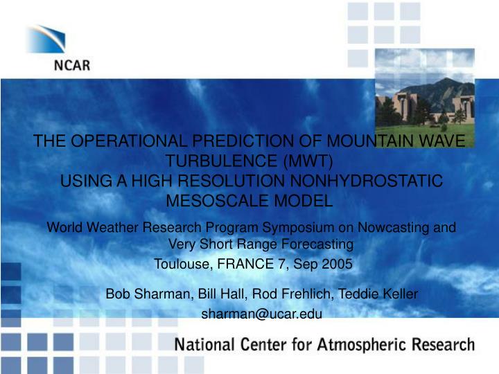
THE OPERATIONAL PREDICTION OF MOUNTAIN WAVE TURBULENCE (MWT)

1. THE OPERATIONAL PREDICTION OF MOUNTAIN WAVE TURBULENCE (MWT) USING A HIGH RESOLUTION NONHYDROSTATIC MESOSCALE MODEL World Weather Research Program Symposium on Nowcasting and Very Short Range Forecasting Toulouse, FRANCE 7, Sep 2005 Bob Sharman, Bill Hall, Rod Frehlich, Teddie Keller sharman@ucar.edu

2. MWT forecasting – “traditional” approach • Identify MWT-prone areas • Use MWT “diagnostics” • Empirical ‘rules-of-thumb” • linear theory • Disadvantages • NWP model is hydrostatic • Waves are nonhydrostatic • Waves and wave “breaking” may be very small scale • Nonlinear effects important • Nonlinear forcing at lower boundary • Wave-wave interactions • Wave-induced critical levels Terra MODIS image 04/04/2004 06 :30 UTC over Crozet Islands, Indian Ocean

3. MWT forecasting – another approach Nested high resolution grid • Mesoscale models have proven capability to model mountain waves (and turbulence?) • Could set up mesoscale model grids over MWT-prone areas • Required resolution ~ 1-3 km horizontally • Uses NWP model for BCs and ICs • Produces 1-6 hr forecasts Outer NWP domain Contours of average annual counts of MOG MWT PIREPs in 40 km2 areas over CONUS based on 10 years worth of PIREPS

4. Case studies • Assess feasibility of using multi-nested model for forecasting MWT • Ability of model to reproduce observed waves and turbulence • Assess timing requirements for operational use • Used two nonhydrostatic models • Clark-Hall anelastic model • AR WRF

5. a) b) c) Example 1: Severe MWT over Alamosa CO 27 Feb 2004 Flight recorder data showing various aircraft parameters as a function of time. Turbulence incident began about 8.47 UTC. Panels show a) wind speed m/s ,b) wind direction (degrees) and c) acceleration in g’s. Water vapor image from MODIS satellite, Feb. 27, 2004 at 5:25 UTC.

6. Domain 3 Domain 1 Terrain contours for the outer domain (domain 1) and inner most domain (domain 3). Red and blue brackets delineate position of domains 2 and 3. Aircraft flight track is represented by red line in domain 3. Example 1: Clark-Hall model setup and results

7. Example 2: Widespread MWT over CO 6 Mar 2004 Water vapor image from MODIS satellite, Mar 6, 2004 at 19:50 UTC.

8. Example 2: WRF ARW Model setup • 24-hr forecast from 0Z • 4 nested domains: 27-9-3-1 km resolution 348x348 @ 1km • 60 vertical levels, avg spacing at 10 km is about 600 m

9. Example 2 results 41 N 37 N

10. Example 2 results (cont.) upper boundary condition

11. Example 2 results (cont.) – edr diagnosis of turbulence (resolved)

12. Timing Model description Δx (km) Δt (sec) nx ny nz Timing (hr) RUC 20 30 301 225 50 0.38 Clark-Hall 12 45 122 122 45 8.57 Alamosa case 4 15 122 122 72 1 5 194 194 72 Clark-Hall 18 60 130 194 45 8.96 6 Mar case 6 20 194 290 74 3 10 194 290 74 WRF 27 120 84 128 61 8.00 6 Mar case 9 40 193 193 61 3 13.3 193 289 61 • Model configurations and timings used in the case studies. The timing is based on one hour of model time using a single 1.3 GHz processor CPU • 32 processors will easily allow operationally useful MWT forecasts

13. Conclusions • MW or lee waves are fairly well understood theoretically • In practice, many facets lead to a “gravity wave soup” that make theory difficult to apply, especially to “breaking” • High resolution simulations seem to reproduce the main features of the waves and “turbulence” • EDR diagnostics capture MWT fairly well for both coarse and high resolution models • Sensitivity studies to model resolutions ongoing • WRF model looks promising once upper boundary condition is fixed

14. Where is MWT? Contours of average annual counts of MOG MWT PIREPs in 40 km2 areas over CONUS based on 10 years worth of PIREPS

15. Expected +2/3 slope Model shape Model deficits edr diagnostic • Eddy dissipation rate or σw (Frehlich and Sharman 2004)

16. Example 2 results (cont.) 41 N 37 N