Download
1 / 16
160 likes | 344 Views
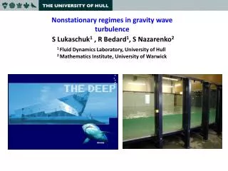
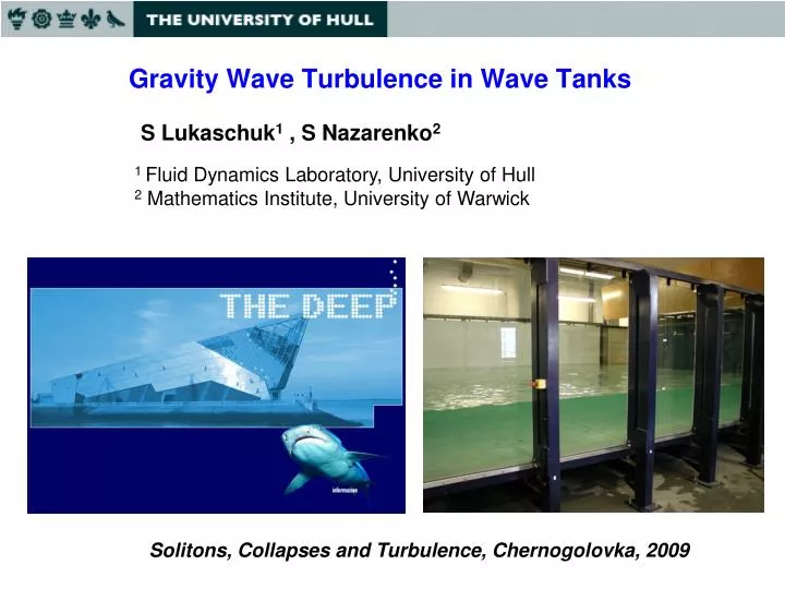
S Lukaschuk 1 , S Nazarenko 2. 1 Fluid Dynamics Laboratory, University of Hull 2 Mathematics Institute, University of Warwick. Gravity Wave Turbulence in Wave Tanks. Solitons, Collapses and Turbulence, Chernogolovka, 2009. Motivation.

E N D
S Lukaschuk1 , S Nazarenko2 1 Fluid Dynamics Laboratory, University of Hull 2 Mathematics Institute, University of Warwick Gravity Wave Turbulence in Wave Tanks Solitons, Collapses and Turbulence, Chernogolovka, 2009
Motivation Knowledge of statistical characteristics of wave turbulence is important for - weather and wave forecasting - prediction of climate change - atmosphere-ocean gas exchange - absorption of solar energy - pollutant transport At the same time there is no clear understanding about mechanisms of wave energy transport within universal interval and dissipation: - different theory predict different energy spectral slope - experimental and statistical results are not sufficient
8-panel Wave Generator C2 CCD Laser C1 12 m M 6 m C1 C2 Experiment C1, C2: Fs=100 Hz 1.3 Mp CCD: Fs=8 Hz M Max water depth 0.9m
Typical spectra Efor small and large wave amplitudes A=3.95 cm (=0.16) A=1.85 cm (=0.074)
Theoretical prediction for spectra of surface gravity waves 1. Poin-like braking events (Phillips) sharp wave crests strong nonlinearity dimensional analysis 2. Propagating braking waves (Kuznetsov) slope breaks occurs in 1D lines wave crests are propagating with a preserved shape 3. Weak turbulence theory (Zakharov random phase (or short correlation length) spatial homogeneity stationary energy flow from large to small scale 4. Finite size effects (Zakharov, Nazarenko) the wave intensity should be strong enough so that non-linear resonance broadening is much greater than the spacing of the k-grid (2/L ).
Spectrum slopes vs the wave spectral density Ef(f is from the inertial interval) Inset: spectral density Efvs the energy dissipation rate =0 “avalanches” and also Phillips =1/3 WTT
Yag Laser x-domain measurements 532 nm 120 mW Dye: Rhodamine 6G Fs=8 Hz ; N=1200 images; Tacq~ 20 min Image size: 1151 x 476 mm Resolution: 0.9 mm/pix
=0.2 k- and -spectra
k- and -slopes • Weak turbulence theory • Breaks (Kuznetsov) • Finite size effects
Increments and Structure Functions - definitions Different types of incoherent and coherent structures (breaks) may lead to the same spectra => to distinguish them we should consider high order correlations - SF. By analogy with hydrodynamic turbulence we introduce differences: which are sensitive to singularities of different order The moments of the increments (SF) are defined as for small l or correspondingly
Asymptotic of the Structure functions For Gaussian statistics and For singular coherent structure with the cross-section For j>1, 0<D<2, 0<a<1 and l ->0 Now suppose that the wave field is bi-fractal and consists of Gaussian incoherent waves and coherent (braking) structures If a<(-1)/2 we expect to see the scaling assosciated with Gaussian rabdom phase waves at small p and coherent structures at larger p.
PDF of 2nd difference in the t- and x-domains l=0.54 cm l=1.1 cm l=2.5 cm l=6.2 cm l=15 cm l=36 cm =30 ms =60 ms =130 ms =290 ms =580 ms Smaller deviation from Gaussian in the t-domain might be due to low propagation speed of the coherent structures leading to their infrequent occurrence in t-domain.
Structure functions in t- and x-domains p=8 . . . p=1 SFs as a function of x or demonstrate power-law scaling in the gravity wave range
SF exponents for t- and x-domains (t) (x) Fit at high p: D=1, a=1.05 D=1.3 , a=0.5 Ku- structures vertical splashes (propagting breaking waves) formed by wave interference
Conclusion • Our experimental data show that spectral exponents are not universal in both -and k –domains and depend on the amplitude of forcing. • We showed that the gravity wave field in the wave tank consists coexisting random and coherent components. • The random waves are captured by the PDF cores and low-order SFs, whereas the coherent wave crests leave their imprints on the PDF tails and on the high-order SFs. • The wave crests themselves consists of structures of different shapes: slow propagating splashes and propagating Ku-type breaks (seen in the t-domain SFs). • We hope that our technique based on SF scalings can be useful in future for analysing the open-sea data, as well as to the future WT theory describing the dynamics and mutual interactions of coexisting random –phased and coherent wave components.