Download
1 / 31
310 likes | 438 Views
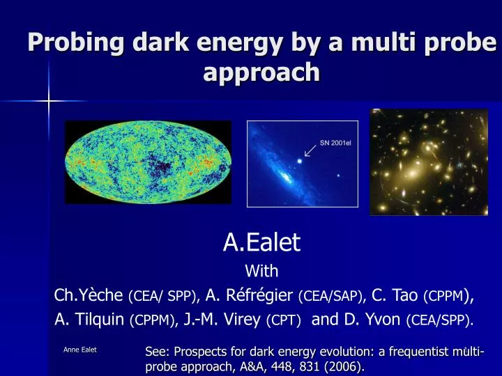
Probing dark energy by a multi probe approach. A.Ealet With Ch.Yèche (CEA/ SPP), A. Réfrégier (CEA/SAP), C. Tao (CPPM ), A. Tilquin (CPPM), J.-M. Virey (CPT) and D. Yvon (CEA/SPP).

E N D
Probing dark energy by a multi probe approach A.Ealet With Ch.Yèche (CEA/ SPP), A. Réfrégier (CEA/SAP), C. Tao (CPPM), A. Tilquin (CPPM), J.-M. Virey (CPT) and D. Yvon (CEA/SPP). See: Prospects for dark energy evolution: a frequentist multi-probe approach, A&A, 448, 831 (2006).
The dark energy question Beyong a precise measure of the standard cosmological parameters.. The question is: • Is acceleration due to the cosmological constant ? • Can we discriminate alternatives? • Cosmological constant • Quintessence are any dynamical component ? • A modification of gravity ? • Some inhomogeneities in LSS What is the best strategy to probe the nature of the dark energy ?
Consistency and precision => many probes… • Background evolution = H(z) => distances measurement • Probing perturbations = g=dr/r/a • 3D weak lensing (DA, and g) • Baryon wiggles (DA) • Supernova Hubble diagram (DL) • Cluster abundance vs z (g) • CMB (DA and g)
But many parameters are strongly correlated • Removing degeneracy without bias => • No direct external prior • Take into account all correlations • (with all cosmological and astrophysical parameters) • In many analyses,basic asumptions are LCDM =flat universe,w=- 1, no DE clustering etc… • Test of consistencies • =>take all correlation into account • => Introduce a systematic error treatment • => need at least 4 different probes Blanchard,Douspis 2004
Résult when wa=0 Dark energyUsing w(z) simulation Wm = 0.3 w0 = -0.7 wa= 0.8 • it is fundamental to have at least 2 free parameters , w and dw/dz • w(z) parametrisation.. w(z) = w0 + (1-a) wa Effect of the parametrisation? • Extraction of wa is difficult Example in supernovae … wa is degenerated with Wm Maor Riess 2004 data
The statistical approach • Developp a flexible tool • A maximum of free parameters • Take all correlation into account • Coherent assumption of models • Can add or remove probes and parameters
Frequentist or Bayesian ?? • Frequentist approach: region of the parameters for which the data have at least a given probability (1-CL) of being described by the model.( Well known by HEP..) • We assume a true value (here (optical depth)) and we measure the “agreement” of the model for this given value. • Bayesian approach: • calculate the probability distribution of the true parameters by assigning probability density functions to all unknown parameters. • The method searches to “predict” a value 1-CL WMAP Team Official paper
impact of a prior • a basic example • Two parameters A and . • A (~82)is measured with TT and TE spectra. • depends only on the first point of the TE spectrum. • Likelihood marginalized for different priors for . • PDF(A) depends a lot on prior choice !
1-CL CL Fitter with Frequentist approach • Principle: • Minimize the 2 • Fix one of the variables, for instance I • Repeat the fit and determine the new minimum • Confidence Level f parameter i is defined by • Extension to 2-D contours with two fixed parameters i and j.
The tools • Minuit as Fitter • Cmbeasy for CMB • Kosmoshow (from A.Tilquin) for SNIa . Minimization after 200-300 call to Cmbeasy. One job per batch (~1h) at CCIN2P3 (IN2P3 computing Center) Flexible can easily add or remove parameter..
A test of faisability .. Use SN and CMB data • Use 1st year WMAP TT and TE spectrum • Use SNIa = 157 SNIa: Riess et al. (2004). • Fit with 9 parameters
The parameters 9 free parameters … • b/m density for baryon/matter • h Hubble constant, • nsspectral index, • reionisation optical depth • A(~82) normalization parameter for CMB (and WL). • Ms0 normalization parameter for SNIa. • ( NB: neutrino masses neglected) • Parameterization of Dark Energy: • Dark Energy perturbations for CMB: 2 options: • No perturbation: DE homogeneous and no clustering • With perturbations: APPLIED only for w>-1
fit results for w0 and wa • Value of w0 smaller than -1.0 are favored • Discrepancy in w0 / strategy for DE perturbation treatment. • Errors significantly be degraded when DE perturbations added.
Comparison with other combinations Seljak et al. (2004) w0 ~ -1 and wa~0. 2) Upadhye et al. (2004) w0 ~ -1.3 and wa~1.2 the 2s discrepancy may be due to a different treatment of DE perturbation in CMB. 1) No DE perturbations 2) DE perturbations for w>-1. Upadhye et al., astro-ph/0411803
can be use forprospectives … 3 scenarii • Today: Reference point • WMAP 1 year • 157 SNIa (Riess 2004). • Mid-term: 2007-2008 • CMB: WMAP + Olimpo (balloon with good resolution and a small field). • SNIa: SNLS (700) +SNFactory (200) +HST (50) • WL: CFHT-LS. (170 deg2) • Long-term:2012-2015 • CMB: Planck • SNIa: SNAP/JDEM (2000 + 300) + 2 % of systematic • WL: SNAP/JDEM 1000 deg2
Some prospectives adding WL on wa Fisher approach on (w0,wa) Add WL information (Icosmo program (A.Refregier)) Simulation of a mid term data WMAP 1 year + Olympo +CFHTLS WL + SNLS SNIA
Expected sensitivity • With ground observations (mid-term), good precision on w0 alone, but not on wa. • Satellite observations (Planck and SNAP) are required to achieve the 0.1 precision on w. • Very impressive sensitivity on other parameters, in particular ns (test of inflationary models).
Expected sensitivity for Long Term Scenario SUGRA -CDM Phantom • precision of the long-term scenario, needed to discriminate models ( here Phantom - CDM – SUGRA). • Sensitivity depends on the position in the w0-wa plane. • In the Long-term scenario, WL gives very promising results (as good as SN+CMB). • However, systematics effects not studied for WL.
FUTURE • Optimizing the tool: • we plan to have a software package allowing contour plots in a few minutes for more than 10 cosmological parameters. • Provide a graphical interface • Preparing a frame • add new probes (BA0, clusters, SZ..) • Work on experimental and theoretical systematic modelization • define benchmark of models for test hypothesis
Conclusion • We have used a frequentist approach to test DE with a combination • We test the methode on current data (WMAP1 year + SNIa), • For the DE evolution, we get: • We have observed a strong effect on (w0, wa) related to the treatment of DE perturbations, which may explain the discrepancies observed in the literature. • Our prospect study demonstrates that we need satellite observations and many probes to achieve a 0.1 sensitivity on wa.
Stronger constraints thanks to correlations • For m-w0 and for w0-wa, we observe • orthogonal correlations between (CMB-WL) • and SNIa • It allows to break the degeneracies. • Actually we have 9-dim correlations, we gain more than the simple 2-dim overlap! • We use the full correlation matrix. 24
Stronger constraints thanks to correlations • For m-w0 and for w0-wa, we observe • orthogonal correlations between (CMB-WL) • and SNIa • It allows to break the degeneracies. • Actually we have 9-dim correlations, we gain more than the simple 2-dim overlap! • We use the full correlation matrix. 26
Error on Cl with Olimpo Cosmic variance Detector performances Cosmic variance Resolution effect • Nominal configurations: • Observed Sky: S=300 deg2 • Detector sensitivity: s=150 Ks1/2 • Number of bolometers: Nbolo= 20 • Observation time: Tobs = 10 days • Resolution: fwhm = 4 arcmin
Error on Cl with Planck • Nominal configurations: • Full Sky, 12 months • 3 Frequencies: 100 / 143 / 217 (GHz) • Sensitivity R= 2.0 / 2.2 / 4.8 (K/K) • Resolution: fwhm = 9.2 / 7.1 / 5.0 arcmin • (Figures extracted from The Planck mission J.A. Tauber • JASR 6394 (2004) )
Examples of 1D Confidence Level Plot WMAP bh2 Scan bh2 : [0.0215, 0.0239]@68% [0.0209, 0.0247]@90% mh2 : [0.130, 0.162]@68% [0.121, 0.174]@90% h : [0.66, 0.75]@68% [0.63, 0.78]@90% A : [0.75, 0.93]@68% [0.70, 1.00]@90% ns : [0.958, 1.013]@68% [0.943, 1.034]@90% : [0.091, 0.0173]@68% [0.068, 0.204]@90% WMAP hScan