Download
1 / 51
510 likes | 535 Views
Explore the concept of linear classifiers for normal distributions, including conditions, empirical results, and graphical analysis. Learn about pairwise linear classifiers, Minsky's Paradox, and Bayes Classification in pattern recognition.

E N D
B. John Oommen A Joint Work with Luis G. Rueda School of Computer Science Carleton University On Optimal Pairwise Linear Classifiers for Normal Distributions
Problem: Find a Linear Classifier (also Optimal) For normal distributions: Believed linear only when covariance matrices equal We found other cases for linear classifiers: Even when covariance matrices Our classifier :Linear and Optimal Found necessary and sufficient conditions Two-dimensional and Multi-dimensional r.v. Pairwise Linear Classifiers
Pattern Recognition : Introduction Diagonalization Bayes Classification Minsky’s Paradox Optimal Pairwise Linear Classifiers Conditions and Classifier for 2-D r.v. Empirical Results Graphical Analysis Conditions and Graphics for d-D r.v. Outline
Linear Classifiers • Discriminant Fn.: Linear or Quadratic Optimal or Non-Optimal • Non-Optimal Approaches: • Fisher’s Approach • The Perceptron Algorithm • Piecewise Recognition Models • Random Search Optimization • Optimal: • Bayes Classifier (but in general quadratic)
Importance of the Problem • Linear Classifiers are easy to implement. • Classification: A simple linear algebraic operation • We have shown that it is POSSIBLE to find a classifier such that: • It is Optimal (Bayesian) • It is Linear • A Pair of Straight Lines (pairwise linear)
1 Or this straight line + y 2 + This straight line x Minsky’s Paradox Also known as: Two-bit parity problem Graphically, Two overlapping classes: 1 and 2 Minsky (1957) showed that it is NOT possible to find a singlelinear classifier.
1 + y 2 + x Pairwise Linear Classifiers Then, we found that the classifier can be a PAIR OF STRAIGHT LINES The classifier is LINEAR, PAIRWISE, and OPTIMAL
1 y 2 x Pairwise Linear Classifiers We even went further …. To a more general case For two overlapping classes We found the necessary and sufficient conditions for a LINEAR, PAIRWISE, and OPTIMAL classifier.
Ex.: Quadratic Functions Roots: x = 1 Roots: x = 1 and x = 3 Every Quadratic Fn. can be factored into: • Quadratic from • Two linear products • All these years, people only considered when two products are the same.
Quadratic Functions (Cases) • Two straight lines: • A single straight line: • An ellipsis: • A hyperbola:
Bayes Classification We have c classes: 1 , 2 , … , c with a priori probabilities: P(1), … , P(c) Given a realized vector, X, Aim: Maximize the a posteriori probability:
Bayes Classification We consider : normal distribution, two classes is the covariance matrix, and M is the mean vector Discriminant function (two classes): p(1| X) = p(2 | X)
Example: Points with the same Mahalanobis distance, or the same probability Normal Distribution (2-D)
Simultaneous Diagonalization • Two normally distributed random vectors : • X1 N( M1 , 1 ) • X2 N( M2 , 2 ) • Orthonormal transformation : • Based on eigen vectors of 1 : 1 • Whitening transformation : • Based on eigen values of 1 : 1 • Result : • X1 N( M1Z , I ) • X2 N( M2Z , 2Z )
Simultaneous Diagonalization • Third transformation : • Orthonormal transformation in the direction of eigen vectors of 2Z : 2 • I is invariant under any transformation • Result : • X1 N( M1Z , I ) • X2 N( M2Z , D) • where D is a diagonal matrix • The axes of the system are in the direction of D
Simultaneous Diagonalization Example : X1 N( M1 , 1 ) X2 N( M2 , 2 ) First transformation :
Simultaneous Diagonalization Second transformation : Third transformation :
y y x x Simultaneous Diagonalization
y y x x Simultaneous Diagonalization
Shifting System Coordinates Theorem : Shifting the system coordinates Two normal random vectors: X 1 and X2 Representing two classes : 1 and 2 X1 and X2can be transformed into Z1 and Z2, where
y y s q - r r x s - s x r p Shifting System Coordinates
I - Diagonalized Classes: 2-D • Optimal Pairwise linear classifiers: • Necessary and Sufficient conditions Theorem : Two normal random vectors: X 1 and X2 The optimal classifier is a pair of straight lines. If and Only if a and b are positive real numbers, s.t.:
y 2 X1 1 1 s 2 - r r x - s X2 I - Diagonalized Classes: 2-D
Diagonalized Classes: Conditions Theorem : Conditions for a and b (r, s : Real): Two normal random vectors: X1 and X2 • The classifier is pairwise linear If and only If a and b satisfy : • a > 1 and 0 < b < 1 , or • 0 < a < 1 and b > 1
Special Cases: 2-D Theorem : Symmetry condition Two normal random vectors: X 1 and X2 It is possible to transform X 1 , X2 into Z 1 , Z2 with: • By doing: • Z 1 = AT X 1 and • Z2 = AT X2 where:
y X1 X2 x Special Cases: 2-D
II - Symmetric Covariances: 2-D Linear Discriminant with Different Means: Theorem : Two normal random vectors: X 1 and X2 The optimal classifier is a pair of straight lines If and Only If for any positive real numbers, a and b: Moreover, if: the condition is:
y X1 1 x 2 2 X2 1 II - Symmetric Covariances: 2-D
III - Minsky’sParadox : 2-D Linear Discriminant with Equal Means: Theorem : Two normal random vectors: X 1 and X2 The optimal classifier is ALWAYS a pair of straight lines.
2 y 1 1 2 x III - Minsky’sParadox : 2-D
Discriminant Function Linear Discriminant with Equal Means: Theorem : Two normal random vectors, X 1 and X2 Discriminant function: Pairwise linear classifier (explicit form):
Discriminant Function Pairwise linear classifier (vectorial form) where:
< > Pairwise Linear Classification General inequality for classification (vectorial form): where: Wiis a weight vector, and wiis a threshold weight.
2 1 1 2 Pairwise Linear Classification
Simulation on Synthetic Data • Taken parameters for a particular case. • Generate 100 trainingsamples. • Learn new parameters from these samples using Maximum Likelihood Estimation Method. • Generate Pairwise classifier with new parameters. • Using old parameters, generate 100 testsamples. • Test the linear classifier with testsamples.
I - Linear Classifier: d-D • Optimal linear classifiers : • Necessary and Sufficient conditions Theorem : Two normal random vectors: X 1 and X2 The Optimal Bayesian classifier is a pair of hyperplanes If and Only If...
(a) (b) (c) I - Linear Classifier: d-D there exists i and j such that:
II - Special Cases: d-D Optimal linear classifier with Different Means: Consider two normal random vectors: X 1 and X2 It is possible to find a pair of hyperplanes as the optimal Bayes classifier If and Only If:
III - Minsky’s Paradox : d-D Consider two normal random vectors: X 1 and X2 The optimal classifier is ALWAYS a pair of hyperplanes.
Parameter Approximation • Problem: Given a real-life training data set, D={X1,…,XN}, Find the parameters 2 that maximizes: The log-likelihood function: Subject to the constraint: Solved numerically using the Lagrange multiplier!
Simulation on Real-life Data • Used the Wisconsin Diagnostic Breast Cancer (WDBC) data set. • Two classes: “benign” and “malignant”. • Taken six features for each sample. • Learn new parameters from 100 samples using “Parameter Approximation”. • Generate Pairwise classifier with new parameters. • Tested Our Classifier using 100 test samples for each class.
Empirical Results • Also tested Fisher’s Classifier with same samples. Class 2% more accurate Classifiers