Download
1 / 15
150 likes | 332 Views
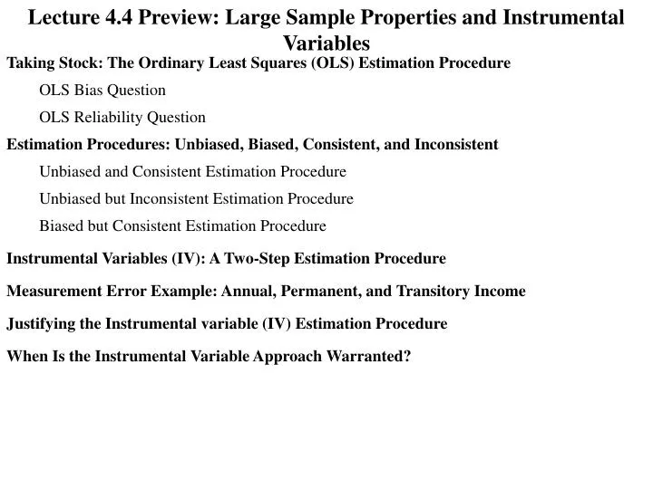
Lecture 4.4 Preview: Large Sample Properties and Instrumental Variables. Taking Stock: The Ordinary Least Squares (OLS) Estimation Procedure. OLS Bias Question. OLS Reliability Question. Estimation Procedures: Unbiased, Biased, Consistent, and Inconsistent.

E N D
Lecture 4.4 Preview: Large Sample Properties and Instrumental Variables Taking Stock: The Ordinary Least Squares (OLS) Estimation Procedure OLS Bias Question OLS Reliability Question Estimation Procedures: Unbiased, Biased, Consistent, and Inconsistent Unbiased and Consistent Estimation Procedure Unbiased but Inconsistent Estimation Procedure Biased but Consistent Estimation Procedure Instrumental Variables (IV): A Two-Step Estimation Procedure Measurement Error Example: Annual, Permanent, and Transitory Income Justifying the Instrumental variable (IV) Estimation Procedure When Is the Instrumental Variable Approach Warranted?
Taking Stock: The Ordinary Least Squares (OLS) Estimation Procedure OLS Bias Question: Are the model’s explanatory variable and error term independent or correlated? Strategy: If we cannot devise an unbiased estimation procedure, we can try to find an estimation procedure that while biased is consistent. Independent Correlated Is the OLS estimation procedure for the value of the coefficient unbiased? No Yes OLS Reliability Question: Are the OLS standard error term premises satisfied or violated? Use an Alternative Approach Satisfied Violated Can the OLS calculation for the coefficient’s standard error be “trusted?” Yes No Use a GLS Approach: Tweak Original Model Is the OLS estimation procedure for the value of the coefficient BLUE? Yes No
Unbiased and Consistent Estimation Procedures Unbiased: Small sample property. The estimation procedure does not systematically underestimate or overestimate the actual value. Formally, the mean of the estimate’s probability distribution equals the actual value. Mean[Est] = Actual Value Informally, when the estimate’s probability distribution is symmetric, the chances that the estimate is greater than the actual value exceed the chances that it is less. Unbiasedness is called a small sample property because it does not depend on the sample size. Unbiasedness depends only of the mean of the estimate’s probability distribution. Consistent: Large sample property. Both the mean and variance of the estimate’s probability distribution are important for consistency: Mean of the estimate’s probability distribution: Either The estimation procedure is unbiased: Mean[Est] = Actual Value or The estimation procedure is biased, but the magnitude of the bias diminishes as the sample size becomes larger. As the sample size approaches infinity the mean approaches the actual value: As Sample Size : Mean[Est] Actual Value Variance of the estimate’s probability distribution: The variance diminishes as the sample size becomes larger As the sample size approaches infinity the variance approaches 0: As Sample Size : Variance[Est] 0
Categorizing Estimation Procedures Does Mean[Est] equal the Actual Value? Yes - Unbiased No - Biased Does Mean[Est] Actual Valueas the sample size ? Yes No Does Var[Est] 0as the sample size ? LabLink 4.2 Yes No LabLink 4.3 Not Consistent After Many, Many Repetitions Mean (Average) Variance Estimation Sample Actual of the Estimated of the Estimated Procedure Size Coefficient Coefficient Values Coefficient Values Consistent OLS 3 2.0 2.0 2.50 OLS 6 2.0 2.0 1.14 Any Two 3 2.0 2.0 7.5 Any Two 6 2.0 2.0 17.3
Revisit Our Friend Clint Random Sample Procedure: Write the name of each individual in the population on a 35 card Perform the following procedure 16 times: Thoroughly shuffle the cards. Randomly draw one card. Ask that individual if he/she is voting for Clint and record the answer. Replace the card. Calculate the fraction of the sample supporting Clint. Is this procedure unbiased? Yes Nonrandom Sample Procedure: Leave Clint’s dorm room and ask the first 16 people you run into if he/she is voting for Clint. Calculate the fraction of the sample supporting Clint. Questions: Compared to the general student population: Are the students who live near Clint are more likely to be Clint’s friend? Yes Are the students who live near Clint more likely to vote for him? Yes Since your starting point is Clint’s dorm room, is it likely that you will poll students who are more supportive of Clint than the general student population? Yes Would you be biasing your poll in Clint’s favor? Yes
Consistent Estimation Procedure Simulation LabLink 4.4 Sampling Population Sample Mean (Average) Magnitude VarianceTechnique Fraction Size Repetitions of Estimates of Bias of Estimates Random .50 16 >10,000 .50 Nonrandom .50 16 >10,000 .56 .06 .015 Nonrandom .50 25 >10,000 .54 .04 .010 Nonrandom .50 100 >10,000 .51 .01 .0025 Is the random procedure unbiased? Yes Is the nonrandom procedure unbiased? No Is the nonrandom procedure consistent? Yes PRS 1 As the sample size increases the magnitude of the bias diminishes. As the sample size increases the variance of the estimates diminishes. The nonrandom procedure is biased, but consistent.
Ordinary Least Squares (OLS) Estimation Procedure, Measurement Error, Bias, and Consistency Even though the ordinary least squares (OLS) estimation procedure for the coefficient value is biased when explanatory variable measurement error is present, perhaps it is consistent. If so, it would be good news. LabLink 4.5 Measurement Error Simulation Actual Mean (Average) Estimation X Sample Coef of the Estimated Magnitude Procedure MErr Var Size Value Coef Values of Bias OLS 50 5 2.0 1.5 0.5 OLS 50 15 2.0 1.3 0.7 OLS 50 25 2.0 1.20.8 Conclusions: When the error terms and the explanatory variables are correlated, the least squares estimation procedure for the coefficient value is not consistent – bad news. is biased – bad news; Question: What should we do when explanatory variable measurement error is present? Strategy: Consider a different estimation procedure. Ideally, that procedure would be unbiased, but failing that perhaps it will be consistent.
Instrumental Variable Approach – A Two Step Procedure Description: An Instrument (Correlated Variable) and Two Regressions Instrument – Correlated Variable: Choose a variable that is correlated with the “problem” explanatory variable (the explanatory variable suffering from measurement error that creates the ordinary least squares (OLS) bias problem). Regression 1 Dependent Variable:“Problem” explanatory variable; Explanatory Variable: Instrument, the correlated variable. Regression 2 Dependent Variable: Original dependent variable Explanatory Variable:Estimate of the “problem” explanatory variable based on the results from regression 1. Claim: While the instrumental variable estimation procedure does not solve the explanatory variable measurement error bias problem, it mitigates the problem. The instrumental variable estimation procedure is consistent. That is, as the sample size becomes larger: The magnitude of the bias becomes less. The variance of the coefficient estimate’s probability distribution becomes less. You may think of this as a “half a loaf is better than none” strategy. Since we cannot devise an unbiased estimation procedure, we are doing the next best thing. We are devising a consistent estimation procedure. We shall justify our claim by using a simulation. Before doing so however, we shall illustrate the “nuts and bolts” of the instrumental variable estimation procedure with an example.
Measurement Error Example: Annual, Permanent, and Transitory Income Permanent income equals what the household earns per year “on average;” loosely speaking, permanent income equals the average of annual income. In some years, the household’s annual income is more than its permanent income, but in other years it is less. Transitory income equals the difference between annual income and permanent income: Sometimes transitory income, IncTranst, is positive, sometimes it is negative, on average it is 0. IncTranst = IncAnntIncPermt or equivalently, IncAnnt = IncPermt + IncTranst Health Insurance Coverage and Permanent Income Theory: Additional state permanent per capita disposable income increases health insurance coverage in the state. Additional permanent income increase health insurance coverage. Model:Coveredt = Const + IncPermIncPermPCt + et Theory:IncPerm> 0 In reality, permanent income and transitory income cannot be observed. The only annual income information is available to assess the theory. Model:Coveredt = Const + IncPermIncAnnPCt + t Theory:IncPerm> 0 Health Insurance Data: Cross section data of health insurance coverage, education, and income statistics from the 50 states and the District of Columbia in 2007. CoveredtAdults (25 and older) covered by health insurance in state t (percent) IncAnnPCt Per capita annual disposable income in state t (thousands of dollars) HSt Adults (25 and older) who completed high school in state t (percent)
Model:Coveredt = Const + IncPermIncAnnPCt + t Theory:IncPerm> 0 Dependent Variable: Covered Explanatory Variable: IncAnnPC EViewsLink Estimated Equation:Covered = 78.6 + .227IncAnnPC Interpretation: We estimate that a $1,000 increase in annual per capita disposable income increases the state’s health insurance coverage by .227 percentage points. Critical Result: The IncAnnPC coefficient estimate equals .227. The positive sign of the coefficient estimate suggests that increases in disposable income increase health insurance coverage. This evidence supports the theory. H0: IncPerm = 0 Disposable income has no effect on health insurance coverage H1: IncPerm > 0 Additional disposable income increases health insurance coverage .0352 = .0176 Prob[Results IF H0 True] = 2 Might this regression suffer from a serious econometric problem, however?
IncAnnPCt = IncPermPCt + IncTransPCt Measurement Error Sometimes transitory income, IncTranst, is positive, sometimes it is negative, on average it is 0. IncAnnPCt = IncPermPCt+ut Mean[ut] = 0 IncPermPCt = IncAnnPCt ut Coveredt = Const + IncPermIncPermPCt + et Theory:IncPerm> 0 = Const + IncPerm(IncAnntut) + et = Const + IncPermIncAnnt IncPermut + et = Const + IncPermIncAnnt + et IncPermut where t = et IncPermut = Const + IncPermIncAnnt + t ut up t down IncAnnt up PRS 2 Explanatory varaible, IncAnnt, and the error term, t, are negatively correlated Whenever the explanatory variable suffers from measurement error and the actual coefficient value is positive, the OLS estimation procedure for the coefficient value is biased downward, toward 0. OLS estimation procedure for the coefficient value is biased downward
Instrumental Variables: An Instrument (a Correlated Variable) and Two Regressions Instrument – Correlated Variable: Choose a variable that is correlated with the “problem” explanatory variable (the explanatory variable suffering from measurement error that creates the ordinary least squares (OLS) bias problem). Adults completing high school (percent), HS Regression 1: Dependent variable: Problem explanatory variable. IncAnnPC Explanatory variable: Instrument, the correlated variable. HS Question: Would you expect education and income to be correlated? EViewsLink PRS 3 Estimated Equation:EstIncAnnPC = 5.27 + .457HS Motivation for Regression 1 Permanent Income Theory: Permanent income depends on education. Model: IncPermPCt = Const + HSHSt + et Theory: Edu > 0 But permanent income is not observable, only annual income is. Model: IncAnnPCt = Const + HSHSt + et Annual income is just permanent income with measurement error. Question: Does dependent variable measure error lead to bias? Answer: No. PRS 4-5 Therefore, Regression 1 provides a “good” estimate of IncPermPC.
Regression 1: Estimated Equation:EstIncAnnPC = 5.27 + .457HS Regression 2: Dependent variable: Original dependent variable Covered Explanatory variable: Estimate of the “problem” explanatory variable based on the results from Regression 1. EstIncAnnPC Estimated Equation:Covered = 39.05 + 1.39EstIncAnnPC Interpretation: We estimate that a $1,000 increase in permanent per capita disposable income increases the state’s health coverage by 1.39 percentage points. Critical Result: The EstIncAnnPC coefficient estimate equals 1.39. The positive sign of the coefficient estimate suggests that increases in permanent disposable income increase health insurance coverage. This evidence supports the theory. The Ordinary Least Squares (OLS) and Instrumental Variables (IV) Estimates IncPerm Estimate SE t-Statistic Tails Prob Ordinary Least Squares (OLS) .227 .105 2.17 .0352 Instrumental Variables (IV) 1.39 .282 4.91 <.0001
Justifying the Instrumental Variable (IV) Estimation Procedure Claim: When explanatory variable measurement error is present the instrumental variables estimation procedure for the coefficient value is biased but consistent. Instrumental Variable Simulation Actual Mean (Average) Variance Estimation X Sample Coef of Estimated Magnitude of Estimated Procedure MErr Var Size Value Coef Values of Bias Coef Values IV 50 5 2.0 3.5 1.5 80 IV 50 15 2.0 2.6 0.6 15 IV 50 25 2.0 2.4 0.4 7 Conclusions: When measurement error is present, the instrumental variable estimation procedure for the coefficient value is biased – bad news; LabLink 4.6 is consistent – good news. Recap: What have we learned about explanatory variable measurement error when the coefficient is nonzero? Both the ordinary least squares estimation procedure and the instrumental variables estimation procedure for the coefficient value are biased. The ordinary least squares estimation procedure is inconsistent also; even when the sample size is large, the average of the estimates does not approach the actual value. The instrumental variables estimation procedure is consistent; when the sample size is large, the average of the estimates does approach the actual value.
When Should Is the Instrumental Variable Approach Warranted? An Empirical Test Instrumental Variable Regression 1: EstIncAnnPC = 5.27 + .457HS Artificial Model: Coveredt = Const + IncPermIncAnnPCt + EstIncAnnEstIncAnnPCt + et Question: If the instrumental variable approach is better than the ordinary least squares approach, should EstIncAnnPC help explain the dependent variable, Covered? Yes Dependent Variable: Covered PRS 6 Explanatory variables: IncAnnPC and EstIncAnnPC EViewsLink Critical Result: The EstIncAnnPC coefficient estimate equals 1.29. The nonzero coefficient estimate suggests that the estimated value of per capita disposable annual income helps explain health insurance coverage. This evidence supports the instrumental variable approach. H0: EstIncAnn = 0 Estimated disposable income has no effect on health insurance coverage H1: EstIncAnn 0 Estimated disposable has no effect on health insurance coverage Prob[Results IF H0 True] = .0001 Question: Does the estimate of income provide significant explanatory power? Yes Question: Is the instrumental variable approach warranted? Yes