Download
1 / 8
80 likes | 189 Views
LEARNING APPLICATION. HEART PACEMAKER. Simplified SCR model. SCR “fires”. Charging phase. As soon as the SCR switches off the capacitor starts charging. Hence, assume. Find R so that the SCR is ready to fire after one second of capacitor charging. %example6p12

E N D
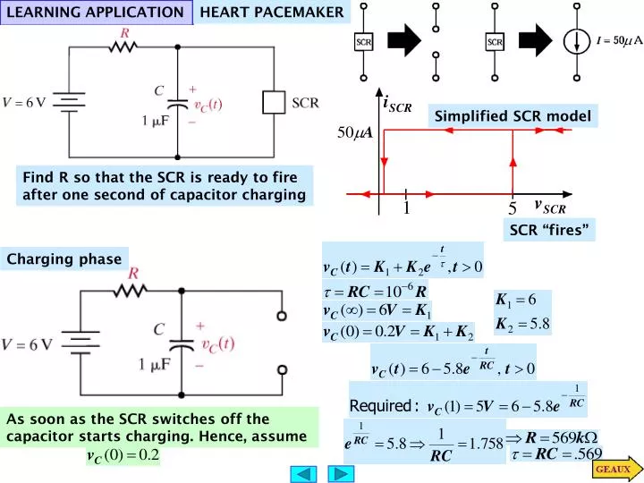
LEARNING APPLICATION HEART PACEMAKER Simplified SCR model SCR “fires” Charging phase As soon as the SCR switches off the capacitor starts charging. Hence, assume Find R so that the SCR is ready to fire after one second of capacitor charging
%example6p12 %visualizes one cycle of pacemaker %charge cycle tau=0.569; tc=linspace(0,1,200); vc=6-5.8*exp(-tc/tau); %discharge cycle. SCR on td=linspace(1,1.11,25); vcd=-22.45+27.45*exp(-(td-1)/tau); plot(tc,vc,'bd',td,vcd,'ro'),grid, title('PACEMAKER CYCLE') xlabel('time(s)'), ylabel('voltage(V)') legend('SCR off', 'SCR on') For SCR turn off THE DISCHARGE STAGE With the chosen resistor discharge starts after one second and the capacitor voltage is 5V
BOOSTER “OFF” PERIOD Inductor releases energy. Capacitor charges BOOSTER “ON” PERIOD Energy is stored in inductor. Capacitor discharges LEARNING EXAMPLE BOOSTER CONVERTER e.g. booster STANDARD DC POWER SUPPLY Inductor current at the beginning of ON period MUST be the same than the current at the end of OFF period
THE “OFF” CYCLE SIMPLIFYING ASSUMPTION: THE OUTPUT VOLTAGE (Vo) IS CONSTANT THE “ON” CYCLE By adjusting the duty cycle one can adjust the output voltage level
LEARNING BY DESIGN Circuit at t=0+ AFTER SWITCHING WE HAVE RLC SERIES For the initial conditions analyze circuit at t=0+. Assume the circuit was in steady state prior to the switching
Mesh plot obtained with MATLAB » s=[[1:9]';[11:19]']; » mesh(t,s,ils') » view([37.5,30]) » xlabel('time(s)'),ylabel('s_1(sec^{-1})') » title('CURRENT AS FUNCTION OF MODES') Ils is a matrix that contains all the computed responses, one per column NOW ONE CAN USE TRIAL AND ERROR OR CAN ATTEMPT TO ESTIMATE THE REQUIRED CAPACITANCE IF FEASIBLE, GET AN IDEA OF THE FAMILY OF SOLUTIONS
Estimate charge by estimating area under the curve For this curve the area is approx. 12 squares %example6p14.m %displays current as function of roots in characteristic equation % il(t)=(60/(s2-s1))*(exp(-s1*t)-exp(s2*t)); % with restriction s1+s2=20, s1~=s2. t=linspace(0,5,500)'; %set display interval as a column vector ils=[]; %reserve space to store curves for s1=1:19 s2=20-s1; if s1~=s2 il=(60/(s2-s1))*(exp(-s1*t)-exp(-s2*t)); ils=[ils il]; %save new trace as a column in matrix end end %now with one command we plot all the columns as functions of time plot(t,ils), grid, xlabel('Time(s)'),ylabel('i(A)') title('CURRENT AS FUNCTION OF MODES')
Applications %verification s1=18.944; s2=20-s1; il=(60/(s2-s1))*(exp(-s1*t)-exp(-s2*t)); plot(t,il,'rd',t,il,'b'), grid, xlabel('time(s)'), ylabel('i(A)') title('VERIFICATION OF DESIGN')