Download
1 / 62
630 likes | 839 Views
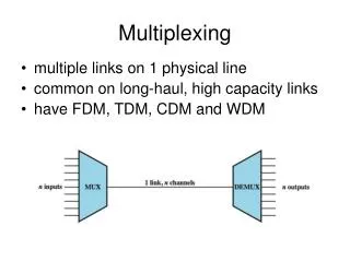
Multiplexing. Multiplexing is the name given to techniques, which allow more than one message to be transferred via the same communication channel. The channel in this context could be a transmission line, e.g. a twisted pair or co-axial cable, a radio

E N D
Multiplexing • Multiplexing is the name given to techniques, which allow more • than one message to be transferred via the same • communication channel. The channel in this context could be a • transmission line, e.g. a twisted pair or co-axial cable, a radio • system or a fibre optic system etc. • A channel will offer a specified bandwidth, which is available for • a time t, where t may . Thus, with reference to the channel • there are 2 ‘degrees of freedom’, i.e. bandwidth or frequency • and time. 1
Multiplexing Now consider a signal The signal is characterised by amplitude, frequency, phase and time. 2
Multiplexing • Various multiplexing methods are possible in terms of the channel bandwidth and time, • and the signal, in particular the frequency, phase or time. The two basic methods are: • Frequency Division Multiplexing FDM FDM is derived from AM techniques in which the signals occupy the same physical ‘line’ but in different frequency bands. Each signal occupies its own specific band of frequencies all the time, i.e. the messages share the channel bandwidth. 2) Time Division Multiplexing TDM TDM is derived from sampling techniques in which messages occupy all the channel bandwidth but for short time intervals of time, i.e. the messages share the channel time. • FDM – messages occupy narrow bandwidth – all the time. • TDM – messages occupy wide bandwidth – for short intervals of time. 3
Multiplexing These two basic methods are illustrated below. 4
Frequency Division Multiplexing FDM • FDM is widely used in radio and television systems (e.g. broadcast radio and TV) and was widely used in multichannel telephony (now being superseded by digital techniques and TDM). • The multichannel telephone system illustrates some important aspects and is considered below. For speech, a bandwidth of 3kHz is satisfactory. • The physical line, e.g. a co-axial cable will have a bandwidth compared to speech as shown next 5
Frequency Division Multiplexing FDM In order to use bandwidth more effectively, SSB is used i.e. We have also noted that the message signal m(t) is usually band limited, i.e. 7
Frequency Division Multiplexing FDM The Band Limiting Filter (BLF) is usually a band pass filter with a pass band 300Hz to 3400Hz for speech. This is to allow guard bands between adjacent channels. 8
Frequency Division Multiplexing FDM For telephony, the physical line is divided (notionally) into 4kHz bands or channels, i.e. the channel spacing is 4kHz. Thus we now have: Note, the BLF does not have an ideal cut-off – the guard bands allow for filter ‘roll off’ in order to reduce adjacent channel crosstalk. 9
Frequency Division Multiplexing FDM Consider now a single channel SSB system. The spectra will be 10
Frequency Division Multiplexing FDM Consider now a system with 3 channels 11
Frequency Division Multiplexing FDM Each carrier frequency, fc1, fc2 and fc3 are separated by the channel spacing frequency, in this case 4 kHz, i.e. fc2 = fc1 + 4kHz, fc3 = fc2 + 4kHz. The spectrum of the FDM signal, M(t) will be: 12
Frequency Division Multiplexing FDM Note that the baseband signals m1(t), m2(t), m3(t) have been multiplexed into adjacent channels, the channel spacing is 4kHz. Note also that the SSB filters are set to select the USB, tuned to f1, f2 and f3 respectively. A receiver FDM decoder is illustrated below: 13
Frequency Division Multiplexing FDM • The SSB filters are the same as in the encoder, i.e. each one centred on f1, f2 and f3 to select the appropriate sideband and reject the others. These are then followed by a synchronous demodulator, each fed with a synchronous LO, fc1, fc2 and fc3 respectively. • For the 3 channel system shown there is 1 design for the BLF (used 3 times), 3 designs for the SSB filters (each used twice) and 1 design for the LPF (used 3 times). • A co-axial cable could accommodate several thousand 4 kHz channels, for example 3600 channels is typical. The bandwidth used is thus 3600 x 4kHz = 14.4Mhz. Potentially therefore there are 3600 different SSB filter designs. Not only this, but the designs must range from kHz to MHz. 14
Frequency Division Multiplexing FDM For ‘designs’ around say 60kHz, = 15 which is reasonable. However, for designs to have a centre frequency at around say 10Mhz, gives a Q = 2500 which is difficult to achieve. To overcome these problems, a hierarchical system for telephony used the FDM principle to form groups, supergroups, master groups and supermaster groups. 15
Basic 12 Channel Group The diagram below illustrates the FDM principle for 12 channels (similar to 3 channels) to a form a basic group. i.e. 12 telephone channels are multiplexed in the frequency band 12kHz 60 kHz in 4kHz channels basic group. 16
Basic 12 Channel Group A design for a basic 12 channel group is shown below: 17
Super Group These basic groups may now be multiplexed to form a super group. 18
Super Group 5 basic groups multiplexed to form a super group, i.e. 60 channels in one super group. Note – the channel spacing in the super group in the above is 48kHz, i.e. each carrier frequency is separated by 48kHz. There are 12 designs (low frequency) for one basic group and 5 designs for the super group. - which is reasonable The Q for the super group SSB filters is Hence, a total of 17 designs are required for 60 channels. In a similar way, super groups may be multiplexed to form a master group, and master groups to form super master groups… 19
Time Division Multiplexing TDM TDM is widely used in digital communications, for example in the form of pulse code modulation in digital telephony (TDM/PCM). In TDM, each message signal occupies the channel (e.g. a transmission line) for a short period of time. The principle is illustrated below: Switches SW1 and SW2 rotate in synchronism, and in effect sample each message input in a sequence m1(t), m2(t), m3(t), m4(t), m5(t), m1(t), m2(t),… The sampled value (usually in digital form) is transmitted and recovered at the ‘far end’ to produce output m1(t)…m5(t). 20
Time Division Multiplexing TDM For ease of illustration consider such a system with 3 messages, m1(t), m2(t) and m3(t), each a different DC level as shown below. 21
Time Division Multiplexing TDM • In this illustration the samples are shown as levels, i.e.V1, V2 or V3. Normally, these voltages would be converted to a binary code before transmission as discussed below. • Note that the channel is divided into time slots and in this example, 3 messages are time-division multiplexed on to the channel. The sampling process requires that the message signals are a sampled at a rate fs 2B, where fs is the sample rate, samples per second, and B is the maximum frequency in the message signal, m(t) (i.e. Sampling Theorem applies). This sampling process effectively produces a pulse train, which requires a bandwidth much greater than B. • Thus in TDM, the message signals occupy a wide bandwidth for short intervals of time. In the illustration above, the signals are shown as PAM (Pulse Amplitude Modulation) signals. In practice these are normally converted to digital signals before time division multiplexing. 23
Time Division Multiplexing TDM A schematic diagram to illustrate the principle for 3 message signals is shown below. Again for simplicity, each message input is assumed to be a DC level. 24
Time Division Multiplexing TDM • Each sample value is converted to an n bit code by the ADC. Each n bit code ‘fits into’ • the time slot for that particular message. In practice, the sample pulses for each • message input could be the same. The multiplexing ADC could pick each input • (i.e. a S/H signal) in turn for conversion. • For an N channel system, i.e.N message signals, sampled at a rate fs samples per • second, with each sample converted to an n bit binary code, and assuming no • additional bits for synchronisation are required (in practice further bits are required) it is • easy to see that the output bit rate for the digital data sequence d(t) is Output bit rate = Nnfs bits/second. 27
School of Electrical, Electronics and Computer Engineering University of Newcastle-upon-Tyne Baseband digital Modulation Prof. Rolando Carrasco Lecture Notes University of Newcastle-upon-Tyne 2005
Bit-rate, Baud-rate and Bandwidth denotes the duration of the 1 bit Hence Bit rate = bits per second All the forms of the base band signalling shown transfer data at the same bit rate. denotes the duration of the shortest signalling element. Baud rate is defined as the reciprocal of the duration of the shortest signalling element. Baud Rate = baud In general Baud Rate ≠ Bit Rate For NRZ : Baud Rate = Bit Rate RZ : Baud Rate = 2 x Bit Rate Bi-Phase: Baud Rate = 2 x Bit Rate AMI: Baud Rate = Bit Rate
Non Return to Zero (NRZ) The highest frequency occurs when the data is 1010101010……. i.e. This sequence produces a square wave with periodic time Fourier series for a square wave, If we pass this signal through a LPF then the maximum bandwidth would be 1/T Hz, i.e. to just allow the fundamental (1st harmonic) to pass.
Non Return to Zero (NRZ) (Cont’d) The data sequence 1010…… could then be completely recovered Hence the minimum channel bandwidth
Return to Zero (RZ) Considering RZ signals, the max frequency occurs when continuous 1’s are transmitted. . This produces a square wave with periodic time If the sequence was continuous 0’s, the signal would be –V continuously, hence
Bi-Phase Maximum frequency occurs when continuous 1’s or 0’s transmitted. This is similar to RZ with Baud Rate = = 2 x Bit rate The minimum frequency occurs when the sequence is 10101010……. e.g. In this case = Baud Rate = Bit rate
Digital Modulation and Noise The performance of Digital Data Systems is dependent on the bit error rate, BER, i.e. probability of a bit being in error. Prob. of Error or BER, Digital Modulation There are four basic ways of sending digital data • The BER (P) depends on several factors • the modulation type, ASK FSK or PSK • the demodulation method • the noise in the system • the signal to noise ratio
Digital Modulation and Noise Amplitude Shift Keying ASK
Digital Modulation and Noise Frequency Shift Keying FSK
Digital Modulation and Noise Phase Shift Keying PSK
System Block diagram for Analysis DEMODULATOR – DETECTOR – DECISION For ASK and PSK
Demodulator-Detector-Decision FOR FSK
Detector-Decision - is the voltage difference between a ‘1’ and ‘0’.
Detector-Decision (Cont’d) ND is the noise at the Detector input. Probability of Error, Hence
Probability density function of noise (*) Using the change of variable
This becomes (**) The incomplete integral cannot be evaluated analytically but can be recast as a complimentary error function, erfc(x), defined by Equations (*) and (**) become
It is clear from the symmetry of this problem that Pe0 is identical to Pe1 and the probability of error Pe, irrespective of whether a ‘one’ or ‘zero’ was transmitted, can be rewritten in terms of v = v1 – v0 • for unipolar signalling (0 and v) • for polar signalling (symbol represented by voltage