Download
1 / 67
670 likes | 677 Views
INDIVIDUAL BEHAVIOR TOWARDS RISK. A- structure of the uncertainty ; Suppose that a farmer is faced with a fertilizer project . STATE OF WORLD 1 2 PLAN RAIN NO RAIN Project A Fertilizer Y A1 = 50 Y A2 =10

E N D
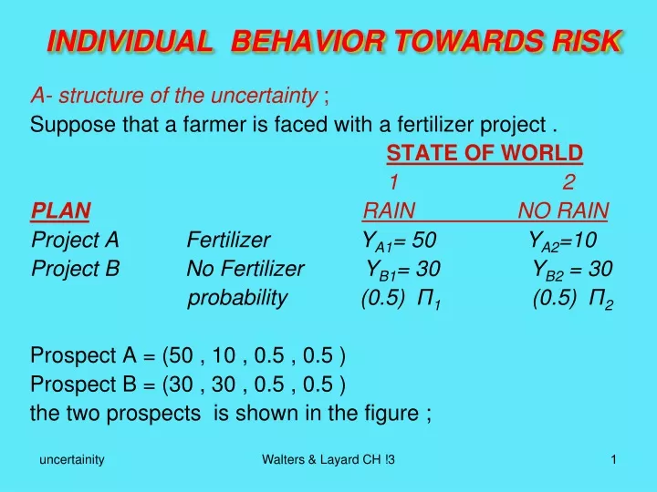
INDIVIDUAL BEHAVIOR TOWARDS RISK A- structure of the uncertainty ; Suppose that a farmer is faced with a fertilizer project . STATE OF WORLD 1 2 PLANRAIN NO RAIN Project A Fertilizer YA1= 50 YA2=10 Project B No Fertilizer YB1= 30 YB2 = 30 probability (0.5) Π1 (0.5) Π2 Prospect A = (50 , 10 , 0.5 , 0.5 ) Prospect B = (30 , 30 , 0.5 , 0.5 ) the two prospects is shown in the figure ; Walters & Layard CH !3
U(Y1 , Y2 , ∏1 , ∏2 ) (Y with ∏1 )=Y1 (Y with ∏2 )= Y2 Walters & Layard CH !3
INDIVIDUAL BEHAVIOR TOWARDS RISK Y2 Certainty line What will be the farmer’s decision We could calculate the expected value of each alternative . C 50 Project B E(Y|A) = Π1 YA1 + Π2 YA2 = (0.5)(50)+(0.5)(10)= 30 E(Y|B) = Π1 YB1 + Π2 YB2 =(0.5)(30)+(0.5)(30)= 30 =certain prospect Farmer choice depends on his preferences . He is able to order all feasible prospects . We could represent his ordering by an ex-ante utility index → V = V ( Y1 , Y2 ; Π1 , Π2 ) 30 If he decides based on expected value , he will be indifferent between choosing A or B . Just like taking a fair gamble . Project A 10 Y1 450 30 10 50 Indifference curve Walters & Layard CH !3
INDIVIDUAL BEHAVIOR TOWARDS RISK however most people are influenced by the spread of possible outcome as well as by the average outcome to be expected . In other words they care about risk . Risk averse person prefer certain outcome to a fair gamble with equal expected value with certain outcome . Risk lover person prefers a gamble to certain outcome with equal expected value . Risk neutral person is indifferent between a gamble and a certain outcome with equal expected value . If needs are the same (taste is the same in rainy and no rain state ) and each state is equally likely , the indifference curve must be symmetric around the 45 degree line . Walters & Layard CH !3
INDIVIDUAL BEHAVIOR TOWARDS RISK If person is risk averse his indifference curve must be convex to the origin , because only this will ensure that he will not take a fair gamble (point A or C ). In other words this will guarantee that point B (certain outcome) is preferred to points A or C . THE EXPECTED UTILITY APPROACH Alternative prospects are ranked according to the expected utility they provide . Our previous general function is now assumed to be in the form of expected utility form ; V(y1 , y2 ; Π1 , Π2) = Π1 U(y1) + Π2U(y2) E(U|A) = Π1 U(yA1) + Π2 U(yA2)= (0.5)U(50) + (0.5)U(10) E(U|B) = (0.5) U(30) + (0.5) U(30) = U(30) He selects point B if E(U|B) > E(U|A) which depends on the shape of the utility function . Walters & Layard CH !3
U(Y) U(50) Risk averse S INDIVIDUAL BEHAVIOR TOWARDS RISK U(30) T (0.5)U(50) + (0.5)U(10) R Risk lover U(10) Risk neutral if individual is risk averse . Point B will be preferred. Y1 Y2 Y 10 30 50 Point B Point A or C Walters & Layard CH !3
INDIVIDUAL BEHAVIOR TOWARDS RISK INSURANCE AND GAMBLING Risk averse person will be willing to pay to avoid risk. Suppose that the current income is 50 . The person will loose 40 if his house burns down . There is a chance of 50-50 of fire. If the person do not insure the house expected utility is measured by the height of point R . The guaranteed income of (30 – TR) will provide him with the equal happiness . A The maximum that he is willing to pay to have a guaranteed income of (30-TR) is (20+TR)=50-(30-TR) when accident does not happen. When accident happens he will receive an insurance payment equal to (20 -TR). In other words with his initial income of 10 he will have (30 – TR) again . So, by paying a premium equal to (20+TR) he will transfer the uncertain prospect A : ( 50 , 10 ; 0.5 ,0.5 ) to a certain prospect of ( 30 – TR , 30 – TR ; 0.5 , 0.5 ) . Walters & Layard CH !3
INDIVIDUAL BEHAVIOR TOWARDS RISK a risk lover person is willing to take fair gamble in contrast to certain outcome . However he will also willing to take unfair gamble provided it is not very unfair. Suppose that the person’s income is 30 and he is offered a bet of 20 units . He will be willing to take it according to the following figure provided that he believes that the probability of wining exceed or equal to (PT/PQ). Suppose that the probability of wining is (PT/PQ) , by taking the bet he will transform the certain prospect of ( 30 , 30 ; 0.5 , 0.5 ) to a uncertain prospect ( 50 , 10 ; PT/PQ , TQ/PQ ) So if probability of winning is between (PT/PQ) and (PN/PQ)the game is unfair (PN/PQ <1/2) but still he accepts the game and prefers it to having of 30 income for certain.(Since he obtains more utility when he accepts uncertain prospect) . Walters & Layard CH !3
U(YA) The risk lover person will pay an amount equal to ST to enter the game . Probability of wining should be greater than (PT/PQ) and smaller than (PN/PQ) for him to accept the game . INDIVIDUAL BEHAVIOR TOWARDS RISK Q U(50) (0.5)U(10) + (0.5)U(50) N T U(30) S P U(10) Y 10 30 50 Walters & Layard CH !3
INDIVIDUAL BEHAVIOR TOWARDS RISK With a small risk (Π=0.3) of a large loss ( house burning ) he will accept a fair insurance. Since U(Y0 – 0.3L ) >[ 0.7u(Y0)+0.3U(Y0 – L)] U U(Y0 + 3S) c 0.75U(Y0- S) + 0.25U(Y0+3S) U(Y0 – S) b Why people both insure and gamble Fridman and Savage postulated a utility function that was concave at low incomes (risk averse at the beginning) and convex at middle income levels (risk lover at middle ages for earning income) and again concave at high income levels risk averse at the final years of life . This kind of utility function could show the following behavior U(Y0) a This does not mean that he will not also take a fair gamble if probability of gain ( ab /ac)=0.25 is less than half and bet is fair {E(x)=3S(0.25) - S(0.75)=0} and the winning (+3s) if successful is larger than the loss ( - s ) if unsuccessful,( stock market ) Y0 = current income U(Y0–L) 0.3(Y0 – L ) + 0.7Y0 Y Y0 - L Y0 + 3S (Y0 – 0.3L)= Y0 - S Walters & Layard CH !3
INDIVIDUAL BEHAVIOR TOWARDS RISK does this really explain the behavior in question ? If we assume that all individuals have the same utility function it implies that gambling will be concentrated in the middle income groups. One alternative approach is to suppose that individuals differ in their utility functions, but each individual has a utility function that is first concave , then convex and after that concave , with convex section beginning at about the level of his current income (Y0). What happens if the convex section extended for any distance . How else we could explain the gambling ? There are two obvious possibilities . First people may overestimate the probability of success. Second , they may enjoy the sensation of gambling for its own sake , as well as the outcomes to which it give rise . Other explanation mat also possible. Walters & Layard CH !3
INDIVIDUAL BEHAVIOR TOWARDS RISK COST OF RISK What is the cost of risk ? How much of his expected income a person faced with a risky prospect would be willing to sacrifice to an insurance company in order to achieve certainty ? We have to find the certainty-equivalent income that gives the same utility as expected utility of uncertain prospect . The cost of risk is the difference between the expected value of a risky prospect and its certainly-equivalent income. The cost of risk will be equal to the distance equal to TR in slide no 5 . The more utility curve is concave (the higher is the degree of risk aversion) , the greater is the cost of risk . It is useful to have a appropriate measure for the cost of risk . Walters & Layard CH !3
INDIVIDUAL BEHAVIOR TOWARDS RISK Very small Cost of risk could be defined as following ; U(YE – C ) = ∑i=1NΠi U (Yi) N = possible state of nature ∑i=1NΠi U (Yi) (BR in slide 6 ) C= (TR in slide 6 ) YE= expected income (point B slide 6) (YE – C ) = the certain income giving utility equal to the expected utility of the risky prospect . If C is reasonably small , and using the Taylor series ; U(YE – C ) ≈ U(YE) – U’(YE) C + U”(YE)(C2/2) C = ( YE – Y ) , Y =(YE – C )= certain income U( YE – C ) = U(Y) U(YE – C )=U(Y)≈U(YE)-U’(YE) (YE-Y)+(1/2)U”(YE)(YE-Y)2 E{U(Yi)}=∑i=1NΠi U (Yi)=∑i=1NΠi U(YE)+U’(YE){∑i=1NΠi (Yi-YE)} + (1/2)U”(YE) ∑i=1NΠi (Y-YE)2 ∑i=1NΠi U (Yi) = U(YE)+U’(YE) (0)+ (1/2) U”(YE) VAR (Y) Walters & Layard CH !3
INDIVIDUAL BEHAVIOR TOWARDS RISK ∑i=1NΠi U (Yi) = U( YE – C) = U(YE) – U’(YE) C + U”(YE)(C2/2) If C is very small then C2 ≈ 0 , so ; ∑i=1NΠi U (Yi) =U(YE) – U’(YE) C , then ; U(YE) – U’(YE) C =U(YE) + (1/2) U”(YE) VAR (Y) C ≈ - (1/2) U”(YE) VAR (Y) / U’(YE) Risk premium= (C/YE) = fraction of expected income that a person would be wiling to sacrifice for the sake of certainty . (C/YE ) ≈{ - U”(YE)YE / 2U’ (YE) } { VAR (Y) / YE2 } C ≈{ - U”(YE)/ 2U’ (YE) } { VAR (Y) } For small VAR ( where YE is small enough) , the cost of risk ( C ) is proportional to the variance of income and risk premium ( C/YE ) is proportional to the coefficient of variation squared . Walters & Layard CH !3
INDIVIDUAL BEHAVIOR TOWARDS RISK -(U”/U’) = degree of absolute risk = Pratt measure. -(U”/U’)YE =degree of relative risk aversion=(dU’/dYE )(YE/U’) Which is equal to the elasticity of the marginal utility of income . The faster the marginal utility of income falls , the more risk averse is the person , so the greater is the cost of risk . RISK POOLING AND RISK SPREADING There are two major mechanism by which the cost of risk could reduce . Risk spreading and risk pooling . 1-RISK POOLING there is a large number of individuals (n) all whom faces the same risky prospect . Each person income is a random variable with a given distribution and the distribution is the same for all individuals. the distribution of each person’s income is independent of the distribution of each other person’s income.( every one face's the same probability of his house being set into fire , but the accident of one’s house being set into fire is independent of the other one.) Walters & Layard CH !3
INDIVIDUAL BEHAVIOR TOWARDS RISK Suppose that n individual get together and pool their income, agreeing that each shall draw the average income. ΣYi /n = (Y1 + Y2 + ….+ Yn )/n → Yi = ΣYi /n , Yi = the ith individual income distribution i=1,2,3….n The variance in their total income is the same whether the income are pooled or not . Since all income distributions are independent from each other and have the same variance. Pooled ; Var(Y1 +.. Yn )=Var (Σ Yi /n +….. Σ Yi /n ) Var ( n Σ Yi /n ) = Var (Σ Yi) = n Var ( Yi ) Unpooled Var (Y1 + Y2 + Y3 ) = Var (Σ Yi ) = n Var ( Yi ), But the variation in individual income is reduced . Originally individual i receives Yi and his variance in income is Var (Yi) After pooling the income, each receive ΣYi /n and the variance of each individual income is Var (Σ Yi /n) = 1/n2 Var Σ Yi = (1/n2 ) n Var (Yi ) =n/n2 Var(Yi )= 1/n Var(Yi ) When n → ∞ , then Var (Σ Yi /n) =0 Walters & Layard CH !3
INDIVIDUAL BEHAVIOR TOWARDS RISK If n identically distributed and independent income distribution are pooled , the variance of average income tends to converge to zero as n tends to infinity in other words ; C = cost of risk ≈ {- U”(YE )/ 2U’(YE )} VAR (Y) = 0 example of risk pooling are friendly societies and business merges . 2 - RISK SPREADING This is spreading one given income distribution over more than one person . If a risky project is undertaken by one person , the cost of risk is ; C = (-U”/2U’)Var(Y) . But if the same risky project is undertaken jointly by a group of n person who agrees to divide the proceeds equally, then, Y/n = income of each one who participate in the project . Walters & Layard CH !3
INDIVIDUAL BEHAVIOR TOWARDS RISK Ci = cost of risk for each individual= (-U”/2U’)Var(Y/n) =(-U”/2U’n2) Var(Y) Total cost of risk= C = n Ci = (-U”/2U’ n){Var(Y)} If n → ∞ , then C = 0 . This is the base of joint stock company . The net benefit of most public sector projects can be spread over a large enough number of people , for the cost of risk is negligible . 3-THE COST OF COVARIANC So far only one source of uncertainty is postulated . More realistic picture of the problem is as following , in which there are more than one source of uncertainty . Walters & Layard CH !3
INDIVIDUAL BEHAVIOR TOWARDS RISK STATE 1 STATE 2 PLANRAIN NO RAIN A ; FERTILIZER50 10 B ; NO FERTILIZER30 20 How does this affect the cost of risk . Farmer’s income (Y) = income without fertilizer (X) + return to fertilizer project ( Z) Project cost of risk = what amount of certain return to project ( ZE – C ) would give the same expected utility as the actual project . Σi Πi U(Xi + ZE – C) = ΣiΠi U(Xi + Zi ) X1 = 30 , X2=20 , Z1 =20 , Z2 = -10 , ZE = ½(20) + ½(-10)= 5 ΣiΠi U( Xi + Zi ) = expected utility of the total income of actual project (like BR in slide 6 ) Walters & Layard CH !3
INDIVIDUAL BEHAVIOR TOWARDS RISK Σi Πi U(Xi + ZE – C) = expected utility of certain value of total equivalent income (income without fertilizer in each state plus expected return to the project minus cost of risk . Like YE – C in slide 6 ). As it is noted the procedure is the same as before (slide 6). The only difference is that we have two states of the world ( x=1 , x=2 ) and the same analysis should be repeated in each state noting that in each state (which is one source of uncertainty ) income without fertilizer is given and return to fertilizer is another source of uncertainty. Using the Taylor series as before it could be shown that we will get ; C ≈ ( -U”/2U’) [ VAR(Z) + 2 COV(X , Z) ] If COV(X , Z) =0 , C ≈ ( -U”/2U’) [ VAR(Z)] as before If COV(X , Z) >0 ,|C| is higher than before .Cost of risk is greater if COV(X , Z) <0 , ,|C| is lower than before . Cost of risk is lower Walters & Layard CH !3
INDIVIDUAL BEHAVIOR TOWARDS RISK Consider the following example ; RAIN NO RAIN PLAN A; FERTILIZER50 10 B; TUBE WELL 20 40 C; NUTRAL30 20 PROBABILITY0.5 0.5 Return to project A 20 -10 Return to project B -10 20 Neutral (neither) 30 20 Walters & Layard CH !3
INDIVIDUAL BEHAVIOR TOWARDS RISK as it is seen the project B will be chosen since COV(X,Z) <0 . When certain income is high , return is low and vice versa . The cost of risk of a project depends on its contribution to the variance of total income , and hence not only on its own variance but on its covariance with other elements of income . MEAN VARIANCE ANALYSIS AND PORTFOLIO SELECTION This section concerns with single investor choice of optimum portfolio . We assume that the investor only cares about the mean and variance of his income . V = V ( YE , var (y) ) , where YE is expected income or mean income .Using Taylor expansion ; ∑i=1NΠi U (Yi) ≈ U(YE) + (1/2) U”(YE) VAR (Y), (slide no. 13) Utility function V could be written in an expected form ; V=f{EU(Y)}= f{ ∑i=1NΠi U (Yi) }=f{ U(YE)+(1/2) U”(YE)VAR (Y) ,} Walters & Layard CH !3
INDIVIDUAL BEHAVIOR TOWARDS RISK For exact reconciliation of V function with E(U) , one or both of the following conditions must hold ; 1 – utility function should be quadratic , 2 – each security in the portfolio has a normal distribution. 1- quadratic utility function U(Y) = a + bY – cY2 E[U(Y)]=a + b E(Y) – cE(Y2), var (y) = E(y – yE)2 =E(y2) – yE2 E[U(Y)] = a + b YE – c [ yE 2 + var (y) ] This implies that for sufficiently high incomes utility falls as income rise (cY2 > a+bY ). If Y is high → (cY2 > a+bY) → U(Y) ↓ This means that U’ (MUy = b – 2cy) should be decreasing or U” should be negative . This means that if there is one risky asset and a safe one, the investor will hold less of the risky asset as he gets richer. If Y is high → ( cE(Y2)> bE(Y) ) → E[U(Y)] ↓ Walters & Layard CH !3
INDIVIDUAL BEHAVIOR TOWARDS RISK Common observation does not suggest that risk is inferior in the sense that the rich people tends to hold less of the risky asset ( higher yield portfolio ) than poor. So the quadratic function may not be a good example . 2- normal distribution for each security The ith security with normal distribution ; µi = mean of the ith security , σi2 = variance of ith security , σij = the covariance with the jth security . ai = number of the security of type i µ = ∑i aiµi = mean total income the investor expect . σ2 = ∑i ∑j aiajσij = variance of total income . Distribution of total income is normal with µ and σ2 as mean and variance. There will be different ai with different portfolio , but all will have normal distribution . So all possible distribution will have the same shape except for the mean and variance .so, The investor only concerned with mean and variance of the portfolio . From the two portfolio with the same variance ,σ2, the one with higher mean (µ) will be chosen by a risk averse person . To define the opportunity set the investor needs to know for each σ2 , the maximum µ available . Walters & Layard CH !3
INDIVIDUAL BEHAVIOR TOWARDS RISK suppose that there are two divisible securities ,X,Z. one unit of each will cost the investor his whole wealth. We will expect that the market to insure that the more risky security has a higher mean return . Suppose that the investor puts halfof his wealth on X and the other half onZ security . In this way ,the mean and variance of the portfolio is as following; µ = (µx + µZ)/2,σxz2 = (1/2)2 σx2 + (1/2)2 σZ2 + 2(1/2)(1/2)σxz Rxz = (σxz) / (σx σz) < 1 2(1/2)(1/2) (σxz) < 2(1/2)(1/2) (σx σz) (1/2)2 σx2+(1/2)2 σZ2+2(1/2)(1/2)σxz<(1/2)2 σx2+(1/2)2 σZ2+2(1/2)(1/2) (σx σz) σxz2 < (1/2 σx + 1/2 σZ)2 → σxz < (1/2 σx + 1/2 σZ) →looking at the figure we will see that the frontier of the opportunity set is concave . Walters & Layard CH !3
Frontier of the opportunity set Z μz σxz < (1/2 σx + 1/2 σz ) T Set of risky portfolio μ X INDIVIDUAL BEHAVIOR TOWARDS RISK μx P μp σx σxz σz Q M μR= R (½)(σx+σz) Suppose that there is one risk less asset R , yielding OR for sure if all investor’s wealth is placed in that asset . Suppose that he puts half of his wealth on risk less asset , R(μ,0) , and half of his wealth on risky one , P(μp , σp) , then point Q (μq , σq ) will be resulted which is the utility maximization point . σR=0 σp σQ = (½)σp + 0 Walters & Layard CH !3
INDIVIDUAL BEHAVIOR TOWARDS RISK He will never mix point R with any other point (like M) inside the set of risky portfolio except point P (point of tangency). Because mixing point R with point P will expand the opportunity set by the whole dashed area which is larger than any other point . A point on the straight line through point R and P is preferred to any other point below it because it lies on a higer opportunity set. It follows that the investor will always choose a point on line PR . In other words he will put a fraction of his wealth into the risk less asset and a fraction into the risky one (like a1 and a2). This policy will yield him more satisfaction (utility) compared to when he puts all of his income to risky asset ( point P ) . So whatever his utility function is, he will always mix his risky assets in the unique ratio ( a1 ,a2 , corresponding to points P , and R ) with risk less one . Walters & Layard CH !3
INDIVIDUAL BEHAVIOR TOWARDS RISK Separation theorem ; • If there is a riskless asset and conditions 1 and/or 2 is satisfied (1 – utility function should be quadratic , 2 – each security in the portfolio has a normal distribution) and all investors have the same subjective probability distributions, then investors will differ in the amount of wealth they hold in the risky assets, but they will not differ in the fraction of that “risky” wealth devoted to each particular risky asset ( a1 ,a2 , corresponding to points P , and R ). • Experiences do not support this ,because ; • A- people may guess differently about mean and variance. • B- they may start from different historically portfolios and locked in by transaction costs or tax problems. • C- different asset might offer different tax advantages. • D- mean-variance approach might have deficiencies. Walters & Layard CH !3
INDIVIDUAL BEHAVIOR TOWARDS RISK THE EXPECTED UTILITY THEOREM . So far we have assumed that people maximize expected utility and have treated this as a hypothesis to be confirmed or disapproved on the base of evidence . Prospect A ; ( 50 , 10 , 0.5 , 0.5 ) Prospect B ; ( 30 , 30 , 0.5 , 0.5 ) We could write the above prospects in the following way ; Prospect A ; ( 50 , 30 , 10 ; 0.5 , 0 , 0.5 ) Prospect B ; ( 50 , 30 , 10 ; 0 , 1 , 0 ) more generally ; prospect A = ( y1 , y2 , y3 ; Π1A , Π2A , Π3A ) prospect B = ( y1 , y2 , y3 ; Π1B , Π2B , Π3B ) 1-First assumption ; there is a preference ordering among all outcomes ( yi) which is complete and transitive . 2-Second ; there is also a preference ordering among all prospects which is complete and transitive . Since the prospects differ only in their probabilities , we can write the utility function as follows , V = V (Π1 , Π2 , Π3). We will show that it is possible to write the above utility function as follows Walters & Layard CH !3
INDIVIDUAL BEHAVIOR TOWARDS RISK V=V (Π1U1 + Π2U2 + Π3U3 ) Where Ui can be defined as utility of outcome yiand also the probability as shown in the following ; If (y ; y1…..yn ) ynis best and y1 is worst ,then by Von-Nweman & Morgeneshtern theorem ; For each yi , there exist probability Πiin such a way that ; U(yi) = Πi u(yn ) + (1- Πi ) u(Y1 ) Yi = certain income , { Πi u(y1) + (1- Πi ) u(yn)} = the utility of the lottery winning y1 with probability Πi and yn with probability (1 – Πi ) . If u(y1) = 0,u(yn) = 1 , then U(yi)= Πi , { Ui = Πi , utility index} Lets take the best and worst possible outcome (y1 , y3 ) and ask for each outcome (y1 , y2 , y3 ), the following question ; At what probability (Ui = Πi )would he indifferent between Yi ( i=1,2,3 ) for certain and a lottery offering y1 with probability Ui= Πi and offering y3 with a probability (1-Ui) U(yi) = { (Ui)U( y1) + (1-Ui) U( y3 ) } , { Ui = Πi } i = 1,2,3 Insisted of having yi ( i= 1,2,3) for certain we could have a lottery yielding y1 with probability Ui ( i= 1,2,3 ) and y3 with probability (1-Ui) , (i=1,2,3) . As we have mentioned Ui is the probability ( ∏ j) which makes the both sides of the above equation equall. Walters & Layard CH !3
V = V (Π1 , Π2 , Π3 ). U(Y3) utility Instead of having y2 with probability Π2 , we could replace Y1 with probability Π2U2 and Y3 with probability Π2(1-u2), so Π2U(y2 ) = Π2 { (U 2)U( y1) + (1-U 2) U( y3 ) } V (Π1,Π2,Π3 )=V(Π1+Π2U2 , Π2(1-U2)+ Π3 ) {Πi u(y3) + (1- Πi ) u(y1 )} INDIVIDUAL BEHAVIOR TOWARDS RISK U(Y1) Instead of having y1 with probability Π1 we could replace Y1 with probability Π1U1 and Y3 with probability Π1(1-U1) , so Π1U(y1) = Π1{ (U1)U( y1) + (1-U1 ) U( y3 ) } V (Π1,Π2,Π3 )=V(Π1U1+Π2U2 ,0, Π1(1-U1) + Π2(1-U2)+ Π3). Income Y Y3 Yi Y1 Instead of having y3 with probability Π3 , we could replace Y1 with probability Π3U3 and Y3 with Probability Π3(1-U3), so Π 3 U(y3 ) = Π3 { (U3 )U( y1) + (1-U3 ) U( y3 ) } V (Π1,Π2,Π3 )=V(Π1 U1 + Π2 U2 + Π3 U3 , Π1 (1-U1 ) + Π2 (1-U2 ) + Π3 (1-U3 ) V (Π1,Π2,Π3 )=V(Π1 U1 + Π2 U2 + Π3 U3 , 1 – Π1U1 - Π2U2 – Π3U3 ) { Uiy1 + (1-Ui ) y3 } , { Ui = Πi} Walters & Layard CH !3
INDIVIDUAL BEHAVIOR TOWARDS RISK So prospects are ranked according to their probability of happening times their values summed over all outcomes . In other words according to their expected value . We have to make three more assumptions as follows ; 3- if Yi is preferred to Yj a prospect offering a higher probability of Yi and a lower one for Yj , other things equal , will be preferred . if U(Yi)>U(Yj) and Πi>Πj and E[U(Y)] = Πi U(Yi) + Πj U(Yj) → will be higher 4- Assumption of continuity .for any particular Y1 preferred to Y2 , preferred to Y3 , there is one unique probability (U2) , at which the sure outcome Y2 is indifferent to to the lottery with probability U2 of Y1 and (1-U2) of y3 . What this really means is that For every certain prospect (for example , Y2) , there exist an equivalent probability distribution involving Y1 and Y3 Walters & Layard CH !3
INDIVIDUAL BEHAVIOR TOWARDS RISK 5- Assumption of independence . The evaluation of prospect is not affected if some element in it is replaced by another element which is indifferent to it . In particular , any certain element can be replaced by an uncertain prospect of equal value . This assumption has been criticized . For example , it is said , it may require a high probability (U2) to induce a person to sacrifice Y2 , if Y2 is really certain . But if Y2 is not certain anyway , a smaller probability U2 might be sufficient to compensate him . This argument seems to imply that people are averse to risk not because of their concern about the outcomes of various alternatives, but because they dislike the condition of uncertainty . Walters & Layard CH !3
INDIVIDUAL BEHAVIOR TOWARDS RISK Clearly it can be observed that the ranking of the projects according to ΣiΠi (a+bUi) will be the same as ΣiΠi Ui. Equally the utility indicator can not be subjected to any nonlinear increasing transformation without running the risk of obtaining different ranking . EXPECTED UTILITY THEOREM Given assumption 1-5 , an individual chooses among risky prospects according to ΣiΠiUi where Πi is the probability of outcome i and Ui ( a utility index for outcome) is invariant between prospects and is unique up to a linear transformation. Walters & Layard CH !3
UNCERTAINITY ,MARKET EQILIBRIUM , WELFARE ECONOMIC MARKET EQILIBRIUM AND WELFARE ECONOMICS Marketeven under uncertainty could produce efficient outcome . Assumptions are as follows ; the output (Y) is given in each state of the world , Y1 = 100 , when whether is rainy Y2 = 50 , when whether is not rainy Two individuals with utility function Vi = Vi ( Y1i , Y2i ), i = A, B The problem is to find the efficient consumption bundle That is ; Max VA = VA ( Y1A , Y2A ), ST VB0 = VB ( Y1B , Y2B ), Y2 = Y2A + Y2B Y1 = Y1A + Y1B If we could imagine a market for output in each state , then by the knowledge of chapter one , the Pareto efficiency can be resulted . In this way of analysis social welfare can be judged entirely in terms of individual preferences as they are known before the state of nature is known . So we assume that most people put importance on ex-ante utility as well as ex-post utility . Walters & Layard CH !3
UNCERTAINITY ,MARKET EQILIBRIUM , WELFARE ECONOMIC So in this chapter we have used the notion of ex-ante utility function with two components ; first ;Y1 as income in the bad year (when there is no rain with probability of happening equal to 1/2 ) , second ; Y2 as income in the good year (when there is rain , with probability of happening equal to 1/2) . In this way we can define an indifference curve for individuals A and B . Both individuals are risk-averse and possess convex indifference curve (slide no. 2 ) and individual A who is more risk-averse having the more convex one . In order to find out whether the theory of welfare works in the framework of uncertainty we will examine this in the next slide in the context of Edgeworth-Box diagramm. Walters & Layard CH !3
Certainty line OB Contract curve = efficiency locus Y2=50 β α > β → (Y2/Y1)A > (Y2 /Y1)B A who is more risk-averse than B will receives more in the bad year (no rain , Y2 ) than B . This happens because ICA is more convex and closer to certainty line and point Elies above the certainty line. So theory works. 450 c UNCERTAINITY ,MARKET EQILIBRIUM , WELFARE ECONOMICS ICA E e b f g a ICB 450 α α RTSY1 Y2 OA Y1=100 Walters & Layard CH !3
UNCERTAINITY ,MARKET EQILIBRIUM , WELFARE ECONOMICS Common budget line mA = mB Certainty lines Y2 = 50 OB 450 As it is clear from the figure , price in good year relative to bad year (PY1/PY2 ) is less than one which means that output is cheaper in good year (Y1) when there is not shortage of Y . MARKET FOR CONTINGENT COMMODITIES Let us suppose a market for each of these contingent commodities(Y1,Y2) Let us also suppose that each of the individuals A , and B , have an equal initial endowment of money(mA , mB). A is more risk-averse than B , so efficiency locus , and efficiency equilibrium point ( E) lies above the diagonal . Now we should look for a set of prices which could equalize demand and supply in each state under prefect competition. E P 450 PY1/PY2 = RTSY1Y2<1 OA Y1 =100 Walters & Layard CH !3
UNCERTAINITY ,MARKET EQILIBRIUM , WELFARE ECONOMICS Do these state contingent commodities exist ? Insurance and Stock markets are two good examples . To begin with take the following example with two commodities instead of one commodity . STATE 1 STATE 2 COMMODITY X X1 X2 Y Y1 Y2 In order to find the efficient allocation of X and Y between the two individuals A and B , we could solve the welfare maximization optimization as indicated by the following equations ; Walters & Layard CH !3
UNCERTAINITY ,MARKET EQILIBRIUM , WELFARE ECONOMIC Max VA = Π1 U1A (x1 A,y1 A) + Π2 U2 A (x2 A,y2 A) S.T. VB0 =Π1 U1B (x1B,y1B) + Π2 U2 B (x2 B,y2 B) Px1 x1A + Py1 y1A = m1 A Px2 x2 A + Py2 y2 A = m2 A Px1 x1B + Py1 y1B = m1B Px2 x2B + Py2 y2B = m2B this could be clearly be done through first ; contingent commodity market andsecond; equally in theory the efficient allocation could be found using security market only . Under first schemethe individuals are faced with four prices for contingent commodities(Px1 , Py1 , Px2 , Py2 ) and model could be optimized as mentioned above, and under second one the individuals are faced with ; Walters & Layard CH !3
UNCERTAINITY ,MARKET EQILIBRIUM , WELFARE ECONOMIC 1- a price today for a dollar to be delivered in state 1 , namely P1 , and another price for a dollar to be delivered in state 2 , namely P2 . 2 – correct forecast of four future spot prices ; (P*x1 , P*y1 , P*x2 , P*y2) . Let us consider the second scheme ; The individual first of all allocates his initial wealth between the two securities ; buying q1 securities of the first kind to be spent in the first period , and q2 securities of the second kind to be spent in the second period. So ; p1q1 A + p2q2A = mA p1q1 B + p2q2B = mB in each state the individuals are trying to maximize their utility subject to the budget constraint ; Walters & Layard CH !3
UNCERTAINITY ,MARKET EQILIBRIUM , WELFARE ECONOMIC for individual A ; max U1A ( x1 A , y1 A ) S.T. q1 A = Px1*X1 A + Py1* y1 A max U2 A ( x2 A , y2 A ) S.T. q2 A = Px2 *X2A + Py2* y2 A For individual B ; max U1B ( x1 B , y1 B ) S.T. q1 B = Px1*X1 B + Py1* y1 B max U2 B ( x2 B , y2 B ) S.T. q2 B = Px2 *X2B + Py2* y2 B under what circumstances will the actual bundle consumed be the same under both schemes. We need to have the following equalities ; Walters & Layard CH !3
UNCERTAINITY ,MARKET EQILIBRIUM , WELFARE ECONOMIC (Px1*) P1= Px1 , Px1 = actual price of x in state 1 (Px2*)P2 = Px2 Px2= actual price of x in state 2 (Py1*)P1= Py1 (Py2*)P2= Py2 These equalities are required to fulfill the budget constraint ; p1 q1 A = p1Px1*X1 A + p1Py1* y1 A = Px1 x1A + Py1y1A p2 q2 A = p2Px2* X2 A + p2Py2* y2 A = Px2 x2 A + Py2 y2 A p1 q1 B = p1Px1*X1 B + p1Py1* y1 B = Px1 x1B + Py1y1B p2 q2 B = p2Px2 *X2B +p2Py2* y2 B = Px2 x2 B + Py2y2 B mA = p1 q1 A + p2 q2 A mB = p1 q1 B + p2 q2 B Walters & Layard CH !3
UNCERTAINITY ,MARKET EQILIBRIUM , WELFARE ECONOMIC There is no obvious reason why individuals could forecast the future prices correctly . In other words it can be said that the . Pareto-Optimality will be achieved if there is perfect market for state contingent money payments provided that individuals correctly forecast the structure of product prices. If we forget the diversity of commodities and assume that utility depends on income in each state of nature , clearly the security market can do the same job as contingent commodities market . But we need security markets that can provide each individual with whatever income he chooses in each possible state. Does stock market or security market can do the job ? In order to find out the answer we have to work out the stock market function from the view point of stock holders who are controlling the production decision of the firm. . Walters & Layard CH !3
UNCERTAINITY ,MARKET EQILIBRIUM , WELFARE ECONOMIC PRODUCTION DECISION AND STOCK MARKET. What will be the production criteria under uncertainty. The question can be reduced to the one that will ask how will a productive enterprise (firm) in fact behave so as to maximize the welfare of its owners (share holders or stock holders). Suppose that for a firm there exist a number of possible projects and each combination yields the following net income for firm . NET RETURN STATE 1 STATE 2 PROSPECTS A 50 10 B 60 12 ….. …. …. Walters & Layard CH !3
UNCERTAINITY ,MARKET EQILIBRIUM , WELFARE ECONOMIC The firm’s decision is to maximize the owner’s utility . Let us see what the owner’s utility depends upon. The ith individual is maximizing his expected utility ; MAX : EU(Y) = Σk ΠikUi(yik) , yik = Σj Sij Rjk for each K. Subject to his budget constraint which is equal to S.T. : Σj Sij Mj = Σj Sij0Mj; k ; index for the state of the world yik = income of individual i in the state of K . Sij = individual i th share from j th firm’s income. Rjk = income of j th company in the kth state of the world. Sij0 = the initial share of j th firm belongs to individual i . Mj = the market value of all shares of firm j company . Walters & Layard CH !3
UNCERTAINITY ,MARKET EQILIBRIUM , WELFARE CONOMIC It is clear that the shareholders of a firm will gain in welfare from an increase in the market value Mj of the firm . So how can a firm decide whether a given investment will raise its market value . The answer is clear taking into account the following example ; NET RETURN STATE 1 STATE 2 PROSPECTS A 50 10 B 60 12 …….. …… …….. It is noted from the example that whatever the project does , its income in the two states of the world are in the ratio of 5:1. There will be a determinate market price for an income prospect ( 5 ; 1 ) which will not change if our firm invest in project A or B ( or may be in any other project ) . Thus the firm can use this price as a basis for its evaluation of the project . Walters & Layard CH !3
UNCERTAINITY,MARKET EQILIBRIUM,WELFARE ECONOMIC In cases where a pattern of returns is common enough in the economy to have a well defined price , independent of the firm’s decision , we say that the firm belongs to a risk class . In this case, it maximizes the total value of the firm’s business by evaluating prospects at the price relevant to their risk-class. When one considers the number of possible states of nature and different possible patterns of returns,it seems unlikely that the condition would be generally satisfied . For example if my house burns down , there might be no productive enterprise that experiences an increase in profit to compensate me at the time my house burns down . So I can not insure myself against fire by any pattern of share . Walters & Layard CH !3
UNCERTAINITY ,MARKET EQILIBRIUM , WELFARE ECONOMIC For the share market to be a fully efficient instrument for the allocation of risk , it must be possible to assemble a prospect of whatever proportions is optimal , given the initial wealth . This requires that , if there are n states of nature , there are at least n firms whose incomes are linearly independent To solve this assume that I wish to buy the following particular vector of incomes in each state of nature : (Y10 , Y20 , Y30,…Yn0) . Rjk is the net income of j th firm in the k th state of nature . If there are n firms , and there are n states of nature , this gives us an n by n matrix whose element Rjk show the income of each firm in each state of nature . If this matrix is nonsingular , there must exist a vector of share holdings such as ( S1 , S2 , …. Sn ) where Sj is the fraction of j th firm owned by me , such that I guarantee myself the specified income in each state of nature .this pattern of share holdings is got by solving for (S1 , S2 ,,,, Sn) in the following ; Walters & Layard CH !3
UNCERTAINITY ,MARKET EQILIBRIUM , WELFARE ECONOMIC (Y10 , Y20 , …Yn0) =(S1 , S2 ,,,, Sn) R11 ,,,,,,,,, R1n R21 ,,,,,,,,, R2n …................. Rn1 ,,,,,,,,, Rnn It is essential that at least n firms have linearly independent income vectors . If all productive enterprises have the same income in any two of the relevant states of the world , (whether or not my house burns down ) , then this condition is not satisfied . It seems most unlikely that it would be satisfied . For this reason insurance against personal misadventure cannot be achieved fully through the security market, because the stock market is limited by the requirement that each individual gets the same fraction of a given firm’s income in every state of nature . The “perfect insurance market”is free of this constraintwill do the trick : they will allow us to ensure for ourselves any income in any state of nature . Walters & Layard CH !3