Download
1 / 44
440 likes | 452 Views
Approaching the Physical Limits of Computing. Invited talk, presented at ISMVL 2005 35 th Int’l Symp. on Multiple-Valued Logic (Sponsor: IEEE Computer Society) Friday, May 20, 2005. Abstract of Talk. Fundamental physics limits the performance of conventional computing technologies.

E N D
Approaching the Physical Limits of Computing Invited talk, presented at ISMVL 200535th Int’l Symp. on Multiple-Valued Logic(Sponsor: IEEE Computer Society) Friday, May 20, 2005
Abstract of Talk • Fundamental physics limits the performance of conventional computing technologies. • The energy efficiency of conventional machines will be forced to level off in roughly the next 10-20 years. • Practical computer performance will then plateau as well. • However, all of the proven limits to computer energy efficiency can, in principle, be circumvented… • but only if computing undergoes a radical paradigm shift. • The essential new paradigm: Reversible computing. • It involves reusing energy to improve energy efficiency. • However, doing this well tightly constrains computer design at all levels from devices through logic, architectures, and algorithms. • In this talk, I review the stringent physical and logical requirements that must be met, • if we wish to break through the near-term barriers, • and approach the true physical limits of computing. M. Frank, "Approaching the Physical Limits of Computing"
Moore’s Law and Performance • Gordon Moore, 1975: • Devices per IC can bedoubled every 18 months • Borne out by history! • Some fortuitous corollaries: • Every 3 years: Devices ½ as long • Every 1.5 years: ~½ as much stored energy per bit! • It is that that has enabled us to throw away bits (and their energies) 2× more frequently every 1.5 years, at reasonable power levels! • And thereby double processor performance 2× every 1.5 years! • Increased energy efficiency of computation is a prerequisite for improved raw performance! • Given realistic levels of total power consumption. Devices per IC Year of Introduction M. Frank, "Approaching the Physical Limits of Computing"
Efficiency in General, and Energy Efficiency • The efficiencyη of any process is: η = P/C • Where P = Amount of some valued product produced • and C = Amount of some costly resources consumed • In energy efficiency ηe, the cost C measures energy. • We can talk about the energy efficiency of: • A heat engine: ηhe = W/Q, where: • W = work energy output, Q= heat energy input • An energy recovering process : ηer = Eend/Estart, where: • Eend = available energy at end of process, • Estart= energy input at start of process • A computer: ηec = Nops/Econs, where: • Nops = useful operations performed • Econs= free-energy consumed M. Frank, "Approaching the Physical Limits of Computing"
Trend of Minimum Transistor Switching Energy Based on ITRS ’97-03 roadmaps fJ Node numbers(nm DRAM hp) Practical limit for CMOS? aJ CV2/2 gate energy, Joules Naïve linear extrapolation zJ M. Frank, "Approaching the Physical Limits of Computing"
Some Lower Bounds on Energy Dissipation • In today’s 90 nm VLSI technology, for minimal operations (e.g., conventional switching of a minimum-sized transistor): • Ediss,op is on the order of 1 fJ (femtojoule) ηec≲ 1015 ops/sec/watt. • Will be a bit better in coming technologies (65 nm, maybe 45 nm) • But, conventional digital technologies are subject to several lower bounds on their energy dissipation Ediss,op for digital transitions (logic / storage / communication operations), • And thus, corresponding upper bounds on their energy efficiency. • Some of the known bounds include: • Leakage-based limit for high-performance field-effect transistors: • Maybe roughly ~5 aJ (attojoules) ηec≲ 2×10¹⁷ operations/sec./watt • Reliability-based limit for all non-energy-recovering technologies: • On the order of 1 eV (electron-volt) ηec≲ 6×10¹⁸ ops./sec/watt • von Neumann-Landauer (VNL) bound for all irreversible technologies: • Exactly kT ln 2 ≈ 18 meV ηec≲ 3.5×10²⁰ ops/sec/watt • For systems whose waste heat ultimately winds up in Earth’s atmosphere, • i.e., at temperature T ≈ Troom = 300 K. M. Frank, "Approaching the Physical Limits of Computing"
Reliability Bound on Logic Signal Energies • Let Esig denote the logic signal energy, • The energy involved (transferred, manipulated) in the process of storing, transmitting, or transforming a bit’s worth of digital information. • But note that “involved” does not necessarily mean “dissipated!” • As a result of fundamental thermodynamic considerations, it is required that Esig≲kBTsig ln r (with quantum corrections that are small for large r) • Where kB is Boltzmann’s constant, 1.38×10⁻¹² J/K; • and Tsig is the temperature in the degrees of freedom carrying the signal; • and r is the reliability factor, i.e., the improbability of error, 1/perr. • In non-energy-recovering logic technologies (totally dominant today) • Basically all of the signal energy is dissipated to heat on each operation. • And often additional energy (e.g., short-circuit power) as well. • In this case, minimum sustainable dissipation is Ediss,op≳ kBTenv ln r, • Where Tenv is now the temperature of the waste-heat reservoir (environment) • Averages around 300 K (room temperature) in Earth’s atmosphere • For a decent rof e.g.2×1017, this energy is on the order ~40 kT ≈ 1 eV. • Therefore, if we want energy efficiency ηec > ~1 op/eV, we mustrecover some of the signal energy for later reuse. • Rather than dissipating it all to heat with each manipulation of the signal. M. Frank, "Approaching the Physical Limits of Computing"
The von Neumann-Landauer (VNL) Principle • First alluded to by John von Neumann in 1949. • Developed explicitly by Rolf Landauer of IBM in 1961. • The principle is a rigorous theorem of physics! • It follows from the reversibility of fundamental dynamics. • A correct statement of the principle is the following: • Any process that loses or obliviously erases 1 bit of known (correlated) information increases total entropy by at least ∆S = 1 bit = kB ln 2, and thus implies the eventual dissipation at leastEdiss = kBTenv ln 2of free energy to the environment as waste heat. • where kB = log e = 1.38×10⁻²³ J/K is Boltzmann’s constant • and Tenv = temperature of the waste-heat reservoir (environment) • Not less than about room temperature, or 300 K for earthbound computers. implies Ediss ≥ 18 meV. M. Frank, "Approaching the Physical Limits of Computing"
Definition of Reversibility • What does it mean for a dynamical system (either continuous or discrete) to be (time-) reversible? • Let x(t) denote the state of the system at time t. • The universe, or any closed system of interest (e.g. a computer). • Let Ft→u(x) be the transition relation operating between a given two times t and u; i.e., x(u) = Ft→u[x(t)]. • Determined by the system’s dynamics (laws of physics, or a FSM). • Then the system is called “dynamically reversible” iff Ft→u is a one-to-one function, for any times (t, u) where u > t. • That is, t >u: ¬ x1x2: Ft→u(x1) = Ft→u(x2). • That is, no two distinct states would ever go to the same state over the course of a given time interval. • The definition implies determinism, if we also allow u < t. • A reversible system is deterministic in the reverse time direction. M. Frank, "Approaching the Physical Limits of Computing"
Nondeterministic,irreversible Deterministic,irreversible Nondeterministic,reversible Deterministic,reversible Types of Dynamics WEAREHERE M. Frank, "Approaching the Physical Limits of Computing"
Physics is Reversible! • All of the successful models of fundamental physics are expressible in the Hamiltonian formalism. • Including: Classical mechanics, quantum mechanics, special and general relativity, quantum field theories. • The latter two (GR & QFT) are backed up by enormous, overwhelming mountains of evidence confirming their predictions! • 11 decimal places of precision so far! And, no contradicting evidence. • In Hamiltonian systems, the dynamical state x(t) obeys a differential equation that’s first-order in time,dx/dt = g(x) (where g is some function) • This immediately implies determinism of the dynamics. • And, since the time differential dt can be taken to be negative, the formalism also implies reversibility! • Thus, dynamical reversibility is one of the most firmly-established, fundamental, inviolable facts of physics! M. Frank, "Approaching the Physical Limits of Computing"
Illustration of VNL Principle • Either digital state is initially encoded by any of N possible physical microstates • Illustrated as 4 in this simple example (the real number would usually be much larger) • Initial entropy S = log[#microstates] = log 4 = 2 bits. • Reversibility of physics ensures “bit erasure” operation can’t possibly merge two microstates, so it must double the possible microstates in the digital state! • Entropy S = log[#microstates] increases by log 2 = 1 bit = (log e)(ln 2) = kB ln 2. • To prevent entropy from accumulating locally, it must be expelled into the environment. Microstates representinglogical “0” Microstates representinglogical “1” Entropy S =log 4 = 2 bits Entropy S′ =log 8 = 3 bits Entropy S =log 4 = 2 bits ∆S = S′ − S= 3 bits − 2 bits= 1 bit M. Frank, "Approaching the Physical Limits of Computing"
Reversible Computing • The basic idea is simply this: • Don’t erase information when performing logic / storage / communication operations! • Instead, just reversibly (invertibly) transform it in place! • When reversible digital operations are implemented using well-designed energy-recovering circuitry, • This can result in local energy dissipation Ediss << Esig, • this has already been empirically demonstrated by many groups. • and even total energy dissipation Ediss << kT ln 2! • This is easily shown in theory & simulations, • but we are not yet to the point of demonstrating such low levels of total dissipation empirically in a physical experiment. • Achieving this goal requires very careful design, • and verifying it requires very sensitive measurement equipment. M. Frank, "Approaching the Physical Limits of Computing"
How Reversible Logic Avoids the von Neumann-Landauer Bound • We arrange our logical manipulations to never attempt to merge two distinct digital states, • but only to reversiblytransform them fromone state to another! • E.g., illustrated is a reversible operationcCLR (controlled CLR) • It and its inverse cSETenable arbitrary logic! logic 00 logic 01 logic 10 logic 11 M. Frank, "Approaching the Physical Limits of Computing"
A Few Highlights Of Reversible Computing History • Charles Bennett @ IBM, 1973-1989: • Reversible Turing machines & emulation algorithms • Can emulate irreversible machines on reversible architectures. • But, the emulation introduces some inefficiencies • Models of chemical & Brownian-motion physical realizations. • Fredkin and Toffoli’s group @ MIT, late 1970’s/early 1980’s • Reversible logic gates and networks (space/time diagrams) • Ballistic and adiabatic circuit implementation proposals • Groups @ Caltech, ISI, Amherst, Xerox, MIT, ‘85-’95: • Concepts for & implementations of adiabatic circuits in VLSI tech. • Small explosion of adiabatic circuit literature since then! • Mid 1990s-today: • Better understanding of overheads, tradeoffs, asymptotic scaling • A few groups begin development of post-CMOS implementations • Most notably, the Quantum-dot Cellular Automata group at Notre Dame M. Frank, "Approaching the Physical Limits of Computing"
Caveat #1 • Technically, to avoid the VNL bound doesn’t actually require that the digital operation must be reversible at the level of the logical states… • It can be logically irreversible if the information in the digital state is already entropy! • In the below example, the non-digital entropy doesn’t change, because the operation is also nondeterministic (N to N), and the transition relation between logical states has semi-detailed balance, so the entropy in the digital state remains constant. • However, such operations just re-randomize bits that are already random! • It’s not clear if this kind of operation is computationally useful. 0 0 Digital bit with unknown value 1 1 Physical dynamics whose precisedetails may be uncertain M. Frank, "Approaching the Physical Limits of Computing"
Caveat #2 • Operations that are logically N-to-1 can be used, if there are sufficient compensating 1-to-N (nondeterministic) logical operations. • All that is really required is that the logical dynamics be 1-to-1 in the long-term average. • Thus, it’s possible to thermally generate random bits and discard them later when we are through with them. • While maintaining overall thermodynamic reversibility. • This ability is useful for probabilistic (randomized) algorithms. logic 0 logic 1 M. Frank, "Approaching the Physical Limits of Computing"
Reversibility and Reliability • A widespread myth: “Future low-level digital devices will necessarily be highly unreliable.” • This comes from a flawed line of reasoning: • Faster more energy efficient lower bit energies high rate of bit errors from thermal noise • However, this scaling strategy doesn’t work, because: • High rate of thermal errors high power dissipation from error correction less energy efficient ultimately slower! • But in contrast, using reversible computing, we can achieve arbitrarily high energy efficiency while also maintaining arbitrarily high reliability! • The key is to keep bit energies reasonably high! • While recovering most of the bit energy… M. Frank, "Approaching the Physical Limits of Computing"
Minimizing Energy Dissipation Due to Thermal Errors • Let perr = 1/rbe the bit-error probability per operation. • Where r quantifies the “reliability level.” • And pok = 1 − perr is the probability the bit is correct • The necessary entropy increase ∆S per op due to error occurrence is given by the (binary) Shannon entropy of the bit-value after the operation: H(perr) = perr log perr-1 + pok log pok-1. • For r >> 1 (i.e., as r → ∞), this increase approaches 0: ∆S = H(perr) ≈ perr log perr-1 = (log r)/r → 0 • Thus, the required energy dissipation per op also approaches 0: Ediss = T∆S ≈ (kT ln r)/r → 0 • Could get the same result by assuming the signal energy Esig = kT ln r required for reliability level r is dissipated each time an error occurs: Ediss = perrEsig = perr(kT ln r) = (kT ln r)/r → 0 as r → ∞. • Further, note that as r → ∞, the required signal energy grows only very slowly… • Specifically, only logarithmically in the reliability, i.e., Esig = Θ(log r). M. Frank, "Approaching the Physical Limits of Computing"
Device-Level Requirements for Reversible Computing • A good reversible device technology should have: • Low manufacturing cost ¢d per device • Important for good overall (system-level) cost-efficiency • Low rate of static power dissipation Pleak due to energy leakage. • Required for energy-efficient storage especially (but also in logic) • Low energy coefficientcE = Ediss/f (energy dissipated per operation, per unit transition frequency) for adiabatic transitions. • Implies we can achieve a high operating frequency (and thus good cost-performance) at a given level of energy efficiency. • High maximum available transition frequency fmax. • Important for those applications in which the latency of serial threads of computation dominates total cost • Important: For system-level energy efficiency, Pleak and cE must be taken as effective global values measuring the implied amount of energy emitted into the outside environment at temperature Tenv. • With an ideal (Carnot) refrigerator, Pleak = StTenvand cE = cSTenv, • Where St = the static rate of leakage entropy generation per unit time, • and cS = Sgen/f adiabatic entropy coefficient, or entropy generated per unit transition frequency. M. Frank, "Approaching the Physical Limits of Computing"
Early Chemical Implementations • How to physically implement reversible logic? • Bennett’s original inspiration: DNA polymerization! • Reversible copying of a DNA strand • Molecular basis of cell division / organism reproduction • This (and all) chemical reactions are reversible… • Direction (forward vs. backward) & reaction rate depends on relative concentrations of reagent and product species affect free energy • Energy dissipated per step turns out to be proportional to speed. • Implies process is characterized by an energy-time constant. • I call this the “energy coefficient” cEt ≡ Ediss,optop = Ediss,op/fop. • For DNA, typical figures are 40 kT ≈ 1eV @ ~1,000 bp/s • Thus, the energy coefficient cE is about 1 eV/kHz. • Can we achieve better energy coefficients? • Yes, in fact, we had already beat DNA’s cE in reversible CMOS VLSI technology available circa 1995! M. Frank, "Approaching the Physical Limits of Computing"
Energy & Entropy Coefficients in Electronics Q R • For a transition involving the adiabatic transfer of an amount Q of charge along a path with resistance R: • The raw (local) energy coefficient is given bycEt = Edisst = Pdisst2 = IVt2 = I2Rt2 = Q2R. • Where V is the voltage drop along the path. • The entropy coefficient cSt = Q2R/Tpath. • where Tpathis the local thermodynamic temperature in the path. • The effective (global) energy coefficient is cEt,eff = Q2R(Tenv/Tpath). • We pay a penalty for low-T operation! M. Frank, "Approaching the Physical Limits of Computing"
Example of Electronic cEt • In a fairly recent (180 nm) CMOS VLSI technology: • Energy stored per min. sized transistor gate: ~1 fJ @ 2V • Corresponds to charge per gate of Q = 1 fC ≈ 6,000 electrons • Resistance per turned-on min-sized nFET of ~14 kΩ • Order of the quantum resistance R = R0 = 1/G0 = h/2q2 = 12.9 kΩ • Ideal energy coefficient for a single-gate transition ~1.4×10⁻²⁶ J/Hz • Or in more convenient units, ~80 eV/GHz = 0.08 eV/MHz! • with some expected overheads for a simple test circuit, calculated energy coefficient comes out to about 8× higher, or ~10−25 J·s • Or ~600 eV/GHz = 0.6 eV/MHz. • Detailed Cadence simulations gave us, per transistor: • @ 1 GHz: P = 20 μW, E = 20 fJ = 1.2 keV, so Ec = 1.2 eV/MHz • @ 1 MHz: P = 0.35 pW, E = 3.5 aJ = 2.2 eV, so Ec = 2.1 eV/MHz M. Frank, "Approaching the Physical Limits of Computing"
Cadence Simulation Results 2LAL = Two-level adiabatic logic • Graph shows power dissipation vs. frequency • in a shift register. • At moderate frequencies (1 MHz), • Reversible uses < 1/100th the power of irreversible! • At ultra-low power (1 pW/transistor) • Reversible is 100× faster than irreversible! • Minimum energy dissipation < 1 eV! • 500× lower than best irreversible! • 500× higher computational energy efficiency! • Energy transferred is still ~10 fJ (~100 keV) • So, energy recovery efficiency is 99.999%! • Not including losses in power supply 1 nJ 100 pJ Standard CMOS 10 aJ 10 pJ 1 aJ 1 pJ Energy dissipated per nFET per cycle 1 eV 100 fJ 2V 100 zJ 2LAL 1.8-2V 1V 10 fJ 10 zJ 0.5V 0.25V kT ln 2 1 fJ 1 zJ 100 aJ 100 yJ M. Frank, "Approaching the Physical Limits of Computing"
A Useful Two-Bit Primitive:Controlled-SET or cSET(a,b) • Semantics: If a=1, then set b:=1. • Conditionally reversible, if the special precondition ab=0 is met. • Note it’s 1-to-1 on the subset of states used • Sufficient to avoid Landauer’s principle! • We can implement cSET in dual-rail CMOS with a pair of transmission gates • Each needs just 2 transistors, • plus one controlling “drive” signal • This 2-bit semi-reversible operation & its inverse cCLR are universal for reversible (and irreversible) logic! • If we compose them in special ways. • And include latches for sequential logic. drive (0→1) a switch(T-gate) b b a M. Frank, "Approaching the Physical Limits of Computing"
Reversible OR (rOR) from cSET • Semantics: rOR(a,b) ::= if a|b, c:=1. • Set c:=1, on the condition that either a or b is 1. • Reversible under precondition that initially a|b → ~c. • Two parallel cSETs simultaneouslydriving a shared output lineimplement the rOR operation! • This type of gate composition was not traditionally considered. • Similarly one can do rAND, and reversibleversions of all operations. • Logic synthesis with theseis extremely straightforward… Hardware diagram a c b Spacetime diagram a’ a a OR b 0 c c’ b’ b M. Frank, "Approaching the Physical Limits of Computing"
CMOS Gate Implementing rLatch / rUnLatch • Symmetric Reversible Latch Implementation Icon Spacetime Diagram crLatch crUnLatch connect in mem in 2 mem in or connect (in) mem in mem • The hardware is just a CMOS transmission gate again • This time controlled by a clock, with the data signal driving • Concise, symmetric hardware icon – Just a short orthogonal line • Thin strapping lines denote connection in spacetime diagram. M. Frank, "Approaching the Physical Limits of Computing"
Example: Building cNOT from rlXOR • rlXOR(a,b,c): Reversible latched XOR. • Semantics: c := ab. • Reversible under precondition that c is initially clear. • cNOT(a,b): Controlled-NOT operation. • Semantics: b := ab. (No preconditions.) • A classic “primitive” operation in reversible & quantum computing • But, it turns out to be fairly complex to implement cNOT in available fully adiabatic hardware technologies… • Thus, it’s really not a very good building block for practical reversible hardware designs! • Of course, we can still build it, if we really want to. • Since, as I said, our gate set is universal for reversible logic M. Frank, "Approaching the Physical Limits of Computing"
cNOT from rlXOR: Hardware Diagram • A logic block providing an in-place cNOT operation (a cNOT “gate”) can be constructed from 2 rlXOR gates and two latched buffers. • The key is: • Operate some of the gates in reverse! Reversiblelatches A B X M. Frank, "Approaching the Physical Limits of Computing"
Θ(log n)-time carry-skip adder S A B S A B S A B S A B S A B S A B S A B S A B G Cin GCoutCin GCoutCin G Cin GCoutCin G Cin GCoutCin G Cin P P P P P P P P PmsGlsPls Pms GlsPls PmsGlsPls Pms GlsPls MS MS LS LS G G GCout Cin GCout Cin P P P P Pms GlsPls Pms GlsPls MS LS G GCout Cin P P Pms GlsPls LS GCout Cin P With this structure, we can do a2n-bit add in 2(n+1) logic levels→ 4(n+1) reversible ticks→ n+1 clock cycles. Hardwareoverhead is< 2× regularripple-carry! Spacetimeoverhead only ~2(n+1)× a conventionalsingle-cycleequivalent. (8 bit segment shown) 3rd carry tick 2nd carry tick 4th carry tick 1st carry tick M. Frank, "Approaching the Physical Limits of Computing"
32-bit Adder Simulation Results 20x better perf.@ 3 nW/adder 1V CMOS 1V CMOS 0.5V CMOS 0.5V CMOS 2V 2LAL, Vsb=1V 2V 2LAL, Vsb=1V (All results here are normalized to a throughput level of 1 add/cycle) M. Frank, "Approaching the Physical Limits of Computing"
Technological Challenges • Fundamental theoretical challenges: • Find more efficient reversible algorithms • Or, prove rigorous lower bounds on complexity overheads • Study fundamental physical limits of reversible computing • Implementation challenges: • Design new devices with lower energy coefficients cEt • Design high-quality resonators for driving transitions • Empirically demonstrate large system-level power savings • Application development challenges: • Find a plausible near- to medium-term “killer app” for RC • Something that’s very valuable, and can’t be done without it • Build a prototype RC-based solution prototype M. Frank, "Approaching the Physical Limits of Computing"
Plenty of Room forDevice Improvement Power per device, vs. frequency • Recall, irreversible device technology has at most ~3-4 orders of magnitude of power-performance improvements remaining. • And then, the firm kT ln 2 (VNL) limit is encountered. • But, a wide variety of proposed reversible device technologies have been analyzed by physicists. • With theoretical power-performance up to 10-12 orders of magnitude better than today’s CMOS! • Ultimate limits are unclear. .18µm CMOS .18µm 2LAL k(300 K) ln 2 Variousreversibledevice proposals M. Frank, "Approaching the Physical Limits of Computing"
Limiting Cases of Energy/Entropy Coefficients • Entropy/entropy coefficients in adiabatic “single electronics:” • Suppose the amount of charge moved |Q| = q (a single electron) • Let the path consist of a single quantum channel (chain of states) • Has quantum resistanceR = R0 = 1/G0 = h/2q2 = 12.9 kΩ. • Then cE = h/2 = 2.07 meV/THz (very low!) • If path is at Tpath = Troom = 300 K, then cS = 0.08 k/THz. • For N× better efficiency than this, let the path consist of N parallel quantum channels. N×lower resistance. • What about systems where resistive models may not apply? • E.g., superconductors, photonics, etc. • A more general and rigorous (but perhaps loose) lower bound on the energy coefficient in all adiabatic quantum systems is given by the expression cE ≥ h2/4Egt, • where Eg = energy gap between ground & excited states, • and t = time taken for a single orthogonalizing transition • Ex.: Let Eg = 1 eV, t = 1 ps. Then cE ≥ 4.28 μeV/THz. M. Frank, "Approaching the Physical Limits of Computing"
Requirements for Energy-Recovering Clock/Power Supplies • All known reversible computing schemes require a periodic global signal that synchronizes and drives adiabatic transitions. • For good system-level energy efficiency, this signal must oscillate resonantly and near-ballistically, with a high effective quality factor. • Several factors make the design of a satisfactory resonator quite difficult: • Need to avoid uncompensated back-action of logic on resonator • In some resonators, Q factor may scale unfavorably with size • Effective quality factor problem • There’s no reason to think that it’s impossible to do… • But it is definitely a nontrivial hurdle, that we need to face up to, pretty urgently… • If we want to make reversible computing practical in time to avoid an extended period of stagnation in computer performance growth. M. Frank, "Approaching the Physical Limits of Computing"
The Back-Action Problem • The ideal resonator signal is a pure periodic signal. • A pretty general result from communications theory: • A resonator’s quality factor is inversely proportional to its signal bandwidth B. • E.g., for an EM cavity w. resonant frequency ω0, • the half-maximum BW is B = ∆ω = ω0/(2πQ) [1]. • Thus Q∞ B 0. • There must be little or no information in the resonator signal! • However, if the logic load being driven varies from on cycle to the next, • whether due to data-dependent variations, • or structural variations (different amounts of logic being driven per cycle) • this will tend to produce impedance nonuniformities, which will lead to nonuniform reflections of the resonator signal • and thereby introduce nonzero bandwidth into that signal. • Even more generally, any departure of resonator energy away from its ideal desired trajectory represents a form of effective energy dissipation! • we must control exactly where (into what states) all of the energy goes! • the set of possible microstates of the system must not grow quickly [1] Schwartz, Principles of Electrodynamics, Dover, 1972. M. Frank, "Approaching the Physical Limits of Computing"
Unfavorable Scaling of Resonator Quality Factor with Size? • I don’t yet have a perfectly clear and general understanding of this issue, but… • In a lot of oscillating systems I’ve looked at, the resonant Q factor may tend to get worse (or at least, not very much better) as the resonator dimensions get smaller. • E.g., in LC oscillators, inductor Q scales inversely to frequency • EM emission is greater at high frequencies • But, the tendency is for low f large coil sizes, not small! • Anecdotal reports from people working in NEMS community… • It can be difficult to get high Q in nanoscale electromechanical resonators • Perhaps due to present difficulty of precision engineering at nanoscale? • Our own experience working with transmission-line resonators • Example: In a cubical EM cavity of length L, • We have 2πQ = L / 8δ, where δ = skin depth. ([1] again) • Skin depth δ = (2πσk)−1/2, where σ = wall conductivity, k = wave #. • So if L is fixed, high Q small δ large k high f low Q in logic! M. Frank, "Approaching the Physical Limits of Computing"
The Effective Quality Factor Problem • Actual quality factor of resonator Q = Eres/Edissr. • Where Eres = energy contained in resonator signal • and Edissr = energy dissipated in resonator per cycle. • But the effective quality factor, for purposes of doing energy-efficient logic transitions is Qeff = Edeliv/Edissr. • Where Edeliv = energy delivered to the logic per transition. • Since 1/Qeff of the logic signal energy is dissipated per cycle. • Thus, Qeff = Q · (Edeliv/Eres). • That is, the effective Q is taken down by the fraction of resonator energy delivered to the logic per cycle. • If a resonator needs to be large to attain high Q, • it may also hold a large amount of energy Eres, • and so it may not have a very high effective Q for driving the logic! M. Frank, "Approaching the Physical Limits of Computing"
(PATENT PENDING, UNIVERSITY OF FLORIDA) Trapezoidal Resonator Concept Moving metal plate support arm/electrode Moving plate Range of Motion Arm anchored to nodal points of fixed-fixed beam flexures,located a little ways away, in both directions (for symmetry) … z y Phase 180° electrode Phase 0° electrode Repeatinterdigitatedstructurearbitrarily manytimes along y axis,all anchored to the same flexure x C(θ) C(θ) 0° 360° 0° 360° θ θ M. Frank, "Approaching the Physical Limits of Computing"
Serpentine spring Front-side view Proof mass Comb drive Back-side view Previous CMOS-MEMS Resonatorsin post-CMOS DRIE process (in use at UF) 150 kHz Resonators M. Frank, "Approaching the Physical Limits of Computing"
PATENT PENDING, UNIVERSITY OF FLORIDA Resonator Schematic Actuator Sensor Sensor Sensor Sensor Actuator M. Frank, "Approaching the Physical Limits of Computing"
Post-TSMC35 AdiaMEMS Resonator PATENT PENDING, UNIVERSITY OF FLORIDA (Coventorware model) Taped out April ‘04 Drivecomb Sensecomb Flexarm M. Frank, "Approaching the Physical Limits of Computing"
Quasi-Trapezoidal MEMS Resonator: 1st Fabbed Prototype • Post-etch process is still being fine-tuned. • Parts are not yet ready for testing… Primaryflexure(fin) Sensecomb Drive comb PATENT PENDING, UNIVERSITY OF FLORIDA M. Frank, "Approaching the Physical Limits of Computing"
Conclusions • Reversible computing will become necessary within our lifetimes, • if we wish to continue progress in computing performance/power beyond the next 1-2 decades. • Much progress in our understanding of RC has been made in the past three decades… • But much important work still remains to be done. • I encourage my audience to join the community of researchers who are working to address the reversible computing challenge. M. Frank, "Approaching the Physical Limits of Computing"