Download
1 / 24
240 likes | 245 Views
This article discusses the use of topological inference in neuroimaging research, focusing on the techniques of random field theory and its application in statistical parametric mapping. It also explores the concepts of peak height, cluster extent, and number of clusters as topological features for inference. The article provides insights into the challenges and benefits of using random field theory in neuroimaging studies.

E N D
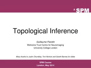
Topological Inference Guillaume Flandin Wellcome Trust Centre for Neuroimaging University College London Many thanks to Justin Chumbley and Tom Nichols for slides SPM Course London, May 2010
Random Field Theory Contrast c
Statistical Parametric Maps mm time frequency mm time 2D time-frequency mm 2D+t scalp-time mm fMRI, VBM,M/EEG source reconstruction mm
Inference at a single voxel u Null Hypothesis H0: zero activation Decision rule (threshold) u: determines false positive rate α Choose u to give acceptable α under H0 Null distribution of test statistic T
Signal Multiple tests u u u u u u If we have 100,000 voxels, α=0.05 5,000 false positive voxels. This is clearly undesirable; to correct for this we can define a null hypothesis for a collection of tests. t t t t t t Noise
Use of ‘uncorrected’ p-value, α =0.1 11.3% 11.3% 12.5% 10.8% 11.5% 10.0% 10.7% 11.2% 10.2% 9.5% Percentage of Null Pixels that are False Positives Multiple tests u u u u u u If we have 100,000 voxels, α=0.05 5,000 false positive voxels. This is clearly undesirable; to correct for this we can define a null hypothesis for a collection of tests. t t t t t t
Family-Wise Null Hypothesis Family-Wise Null Hypothesis: Activation is zero everywhere If we reject a voxel null hypothesis at any voxel,we reject the family-wise Null hypothesis A FP anywhere in the image gives a Family Wise Error (FWE) Family-Wise Error rate (FWER) = ‘corrected’ p-value Use of ‘uncorrected’ p-value, α =0.1 Use of ‘corrected’ p-value, α =0.1 FWE
Bonferroni correction The Family-Wise Error rate (FWER), αFWE, fora family of N tests follows the inequality: where α is the test-wise error rate. Therefore, to ensure a particular FWER choose: This correction does not require the tests to be independent but becomes very stringent if dependence.
Spatial correlations 100 x 100 independent tests Spatially correlated tests (FWHM=10) Discrete data Spatially extended data Bonferroni is too conservative for spatial correlated data.
Random Field Theory Consider a statistic image as a discretisation of a continuous underlying random field. Use results from continuous random field theory. lattice representation
Topological inference Topological feature: Peak height intensity u space non significant local maxima significant local maxima
Topological inference Topological feature: Cluster extent intensity uclus space significant cluster non significant clusters
Topological inference Topological feature: Number of clusters intensity uclus space Here, c=1, only one cluster larger than k.
Terminology Random field f()(spatial stochastic process) Search volume Excursion sets of f over and above the level u: Cluster (extent = # voxels)
No holes Zero or one blob
Expected Euler Characteristic 2D Gaussian Random Field • : search region • ( : volume • ||1/2:roughness (1 / smoothness)
1 2 3 4 5 6 7 8 9 10 1 2 3 4 Smoothness • Smoothness parameterised in terms of FWHM: • Size of Gaussian kernel required to smooth i.i.d. noise to have same smoothness as observed null (standardized) data. FWHM Eg: 10 voxels, 2.5 FWHM, 4 RESELS The number of resels is similar, but not identical to the number independent observations. • Smoothness estimated from spatial derivatives of standardised residuals: • Yields an RPV image containing local roughness estimation.
Corrected p-value for statistic value t Random Field intuition
General form for expected Euler characteristic • t, F & 2 fields • restricted search regions •D dimensions • Random Field: Unified Theory rd (u) :d-dimensional EC density of the field – function of dimension and threshold, specific for RF type: E.g. Gaussian RF: r0(u) = 1- (u) r1(u) = (4 ln2)1/2 exp(-u2/2) / (2p) r2(u) = (4 ln2) u exp(-u2/2) / (2p)3/2 r3(u) = (4 ln2)3/2 (u2 -1) exp(-u2/2) / (2p)2 r4(u) = (4 ln2)2 (u3 -3u) exp(-u2/2) / (2p)5/2
Peak, cluster and set level inference Regional specificity Sensitivity Peak level test: height of local maxima Cluster level test: spatial extent above u Set level test: number of clusters above u : significant at the set level L1 > spatial extent threshold L2 < spatial extent threshold : significant at the cluster level : significant at the peak level
Random Field Theory • The statistic image is assumed to be a good lattice representation of an underlying continuous stationary random field.Typically, FWHM > 3 voxels(combination of intrinsic and extrinsic smoothing) • Smoothness of the data is unknown and estimated:very precise estimate by pooling over voxels stationarity assumptions (esp. relevant for cluster size results). • RFT conservative for low degrees of freedom(always compare with Bonferroni correction).Afford littles power for group studies with small sample size. • A priori hypothesis about where an activation should be, reduce search volume Small Volume Correction: • mask defined by (probabilistic) anatomical atlases • mask defined by separate "functional localisers" • mask defined by orthogonal contrasts • (spherical) search volume around previously reported coordinates
Conclusion • There is a multiple testing problem and corrections have to be applied on p-values (for the volume of interest only (see SVC)). • Inference is made about topological features (peak height, spatial extent, number of clusters).Use results from the Random Field Theory. • Control of FWER(probability of a false positive anywhere in the image): very specific, not so sensitive. • Control of FDR(expected proportion of false positives amongst those features declared positive (the discoveries)): less specific, more sensitive.
References • Friston KJ, Frith CD, Liddle PF, Frackowiak RS. Comparing functional (PET) images: the assessment of significant change. J Cereb Blood Flow Metab. 1991 Jul;11(4):690-9. • Worsley KJ, Marrett S, Neelin P, Vandal AC, Friston KJ, Evans AC. A unified statistical approach for determining significant signals in images of cerebral activation. Human Brain Mapping 1996;4:58-73. • Chumbley J, Worsley KJ , Flandin G, and Friston KJ. Topological FDR for neuroimaging. NeuroImage, 49(4):3057-3064, 2010. • Chumbley J and Friston KJ. False Discovery Rate Revisited: FDR and Topological Inference Using Gaussian Random Fields. NeuroImage, 2008. • Kilner J and Friston KJ. Topological inference for EEG and MEG data. Annals of Applied Statistics, in press. http://www.fil.ion.ucl.ac.uk/spm/doc/biblio/Keyword/RFT.html