Download

1 / 38
1.03k likes | 3.26k Views
Topological insulators. Pavel Buividovich (Regensburg). Hall effect. Classical treatment. Dissipative motion for point-like particles ( Drude theory). Steady motion. Cyclotron frequency. Drude conductivity. Current. Resistivity tensor. Classical Hall effect.

E N D
Topological insulators PavelBuividovich (Regensburg)
Hall effect Classical treatment Dissipative motion for point-like particles (Drude theory) Steady motion
Cyclotron frequency Drude conductivity Current Resistivity tensor Classical Hall effect • Hall resistivity (off-diag component of resistivity tensor) • - Does not depend on disorder • Measures charge/density • of electric current carriers • - Valuable experimental tool
Clean system limit: INSULATOR!!! Importance of matrix structure Naïve look at longitudinal components: INSULATOR AND CONDUCTOR SIMULTANEOUSLY!!! Classical Hall effect: boundaries Conductance happens exclusively due to boundary states! Otherwise an insulating state
Non-relativistic Landau levels Model the boundary by a confining potential V(y) = mw2y2/2 Quantum Hall Effect
Number of conducting states = • no of LLs below Fermi level • Hall conductivity σ ~ n • Pairs of right- and left- movers • on the “Boundary” • NOW THE QUESTION: • Hall state without magnetic • Field??? Quantum Hall Effect
Originally, hexagonal lattice, but we consider square Two-band model, similar to Wilson-Dirac [Qi, Wu, Zhang] Phase diagram m=2 Dirac point at kx,ky=±π m=0 Dirac points at (0, ±π), (±π,0) m=-2 Dirac point at kx,ky=0 Chern insulator [Haldane’88]
Open B.C. in y direction, numerical diagonalization Chern insulator [Haldane’88]
Response to a weak electric field, V = -e E y (Single-particle states) Electric Current (system of multiple fermions) Velocity operator vx,yfrom Heisenberg equations Quantum Hall effect: general formula
Quantum Hall effect and Berry fluxTKNN invariant Berry connection Berry curvature Integral of Berry curvature = multiple of 2π (wave function is single-valued on the BZ) Berry curvature in terms of projectors TKNN = Thouless, Kohmoto, Nightingale, den Nijs
Adiabatically time-dependent Hamiltonian H(t) = H[R(t)] with parameters R(t). For every t, define an eigenstate However, does not solve the Schroedingerequation Substitute Digression: Berry connection Adiabatic evolution along the loop yields a nontrivial phase Bloch momentum: also adiabatic parameter
General two-band Hamiltonian Projectors Berry curvature in terms of projectors • Two-band Hamiltonian: mapping of sphere on the torus, • VOLUME ELEMENT • For the Haldane model • m>2: n=0 • 2>m>0: n=-1 • 0>m>-2: n=1 • -2>m : n = 0 Example: two-band model CS number change = Massless fermions = Pinch at the surface
Along with current, also charge density is generated Response in covariant form Electromagnetic response and effective action Effective action for this response Electromagnetic Chern-Simons = Magnetic Helicity Winding of magnetic flux lines
Consider the Quantum Hall state in cylindrical geometry ky is still a good quantum number Collection of 1D Hamiltonians QHE and adiabatic pumping Switch on electric field Ey, Ay = - Ey t “Phase variable” 2 πrotation ofΦ , timeΔt = 2 π/ LyEy Charge flow in this timeΔQ = σHΔt Ey Ly = CS/(2 π) 2 π = CS Every cycle of Φ moves CS unit charges to the boundaries
More generally, consider a parameter-dependent Hamiltonian Define the current response Similarly to QHE derivation QHE and adiabatic pumping Polarization EM response
Classical dipole moment But what is X for PBC??? Mathematically, X is not a good operator Resta formula: Quantum theory of electric polarization[King-Smith,Vanderbilt’93 (!!!)] Model: electrons in 1D periodic potentials Bloch Hamiltonians a Discrete levels at finite interval!!
Many-body fermionic theorySlater determinant Quantum theory of electric polarization
King-Smith and Vanderbilt formula Polarization = Berry phase of 1D theory (despite no curvature) Quantum theory of electric polarization • Formally, in tight-binding models X is always integer-valued • BUT: band structure implicitly remembers about continuous • space and microscopic dipole moment • We can have e.g. Electric Dipole Moment • for effective lattice Dirac fermions • In QFT, intrinsic property • In condmat, emergent phenomenon • C.F. lattice studies of CME
1D Hamiltonian Particle-hole symmetry Consider two PH-symmetric hamiltoniansh1(k) and h2(k) Define continuous interpolation For Now h(k,θ) can be assigned the CS number = charge flow in a cycle of θ From (2+1)D Chern Insulators to (1+1)D Z2 TIs
Particle-hole symmetry implies P(θ) = -P(2π - θ) • On periodic 1D lattice of unit spacing, • P(θ) is only defined modulo 1 P(θ) +P(2π - θ) = 0 mod 1 • P(0) or P(π) = 0 or ½ Z2 classification • Relative parity of CS numbers • Generally, different h(k,θ) = different CS numbers • Consider two interpolations h(k,θ) and h’(k,θ) • C[h(k, θ)]-C[h’(k,θ)] = 2 n From (2+1)D Chern Insulators to (1+1)D Z2 TIs
Now consider 1D Hamiltonians with open boundary conditions CS = numer of left/right zero level crossings in [0, 2 π] Particle-hole symmetry: zero level at θ also at 2 π – θ Odd CS zero level at π(assume θ=0 is a trivial insul.) Relative Chern parity and level crossing
Once again, EM response for electrically polarized system Corresponding effective action For bulk Z2 TI with periodic BC P(x) = 1/2 Relative Chern parity and θ-term • TI = Topological field theory in the bulk: • no local variation can changeΦ • Current can only flow at the boundary where P changes • Theta angle = π, Charge conjugation only allows • theta = 0 (Z2 trivial) or theta = π(Z2 nontrivial) • Odd number of localized statesat the left/right boundary
Consider the 4D single-particle hamiltonianh(k) Similarly to (2+1)D Chern insulator, electromagnetic response C2 is the “Second Chern Number” (4+1)D Chern insulators (aka domain wall fermions) Effective EM action Parallel E and B in 3D generate current along 5th dimension
In continuum space Five (4 x 4) Dirac matrices:{Γµ , Γν} = 2 δµν Lattice model = (4+1)D Wilson-Dirac fermions In momentum space (4+1)D Chern insulators: Dirac models
Critical values of mass CS numbers (where massless modes exist) (4+1)D Chern insulators: Dirac models Open boundary conditions in the 5th dimension |C2| boundary modes on the left/on the right boundaries Effective boundary Weyl Hamiltonians 2 Weyl fermions = 1 Domain-wall fermion (Dirac) Charge flows into the bulk = (3+1)D anomaly
Consider two 3D hamiltonians h1(k) and h2(k), Define extrapolation “Magnetoelectric polarization” Z2 classification of time-reversal invariant topological insulators in (3+1)D and in (2+1)Dfrom (4+1)D Chern insulators Time-reversal implies P(θ) = -P(2π - θ) P(θ) is only defined modulo 1 => P(θ) +P(2π - θ) = 0 mod 1 P(0) or P(π) = 0 or ½ => C[h(k, θ)]-C[h’(k,θ)] = 2 n
Dimensional reduction from (4+1)D effective action In the bulk, P3=1/2 theta-angle = π Electric current responds to the gradient of P3 At the boundary, Effective EM action of 3D TRI topinsulators • Spatial gradient of P3: Hall current • Time variation of P3: current || B • P3 is like “axion” (TME/CME) • Response to electrostatic field near boundary Electrostatic potential A0
Band inversion at intermediate concentration Real 3D topological insulator: Bi1-xSbx
Consider two 2D hamiltonians h1(k) and h2(k), Define extrapolation h(k,θ) is like 3D Z2 TI Z2 invariant This invariant does not depend on parametrization? Consider two parametrizationsh(k,θ) and h’(k,θ) Interpolation between them (4+1)D CSI Z2TRI in (3+1)D Z2TRI in (2+1D) This is also interpolation between h1 and h2 Berry curvature of φ vanishes on the boundary
Periodic table of Topological Insulators Chern invariants are only defined in odd dimensions
Time-reversal operator for Pauli electrons Anti-unitary symmetry Single-particle Hamiltonian in momentum space (Bloch Hamiltonian) If [h,θ]=0 Consider some eigenstate Kramers theorem
Every eigenstate has a partner at (-k) With the same energy!!! Since θ changes spins, it cannot be Example: TRIM (Time Reversal Invariant Momenta) -k is equivalent to k For 1D lattice, unit spacing TRIM: k = {±π, 0} Assume Kramers theorem States at TRIM are always doubly degenerate Kramers degeneracy
Contact || x between two (2+1)D Tis • kxis still good quantum number • There will be some midgap states crossing zero • At kx= 0, π (TRIM) double degeneracy • Even or odd number of crossings Z2 invariant Z2 classification of (2+1)D TI • Odd number of crossings = odd number of massless modes • Topologically protected (no smooth deformations remove)
Simple theoretical model for (2+1)D TRI topological insulator [Kane,Mele’05]: graphene with strong spin-orbital coupling - Gap is opened - Time reversal is not broken - In graphene, SO coupling is too small Possible physical implementation Heavy adatom in the centre of hexagonal lattice (SO is big for heavy atoms with high orbitals occupied) Kane-Mele model: role of SO coupling
Two edge states with opposite spins: left/up, right/down Spin-momentum locking Insensitive to disorder as long as T is not violated Magnetic disorder is dangerous
Graphene tight-binding model with nearest- and next-nearest-neighbour interactions Topological Mott insulators By tuning U, V1 and V2 we can generate an effective SO coupling. Not in real graphene, But what about artificial? Also, spin transport on the surface of 3D Mott TI [Pesin,Balents’10]
- “Primer on topological insulators”, A. Altland and L. Fritz - “Topological insulator materials”, Y. Ando, ArXiv:1304.5693 - “Topological field theory of time-reversal invariant insulators”, X.-L. Qi, T. L. Hughes, S.-C. Zhang, ArXiv:0802.3537 Some useful references (and sources of pictures/formulas for this lecture :-)