Download
1 / 13
130 likes | 137 Views
LECTURE 03: BASIC SYSTEM PROPERTIES. Objectives: Definition of a System Examples Causality Linearity Time Invariance Resources: MIT 6.003: Lecture 2 Wiki: Causality Wiki: Linear System Wiki: Time Invariant System JHU: LTI Systems. Audio:. URL:. Systems.

E N D
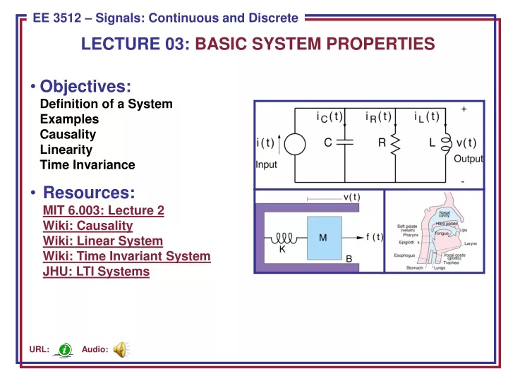
LECTURE 03: BASIC SYSTEM PROPERTIES • Objectives:Definition of a SystemExamplesCausalityLinearityTime Invariance • Resources:MIT 6.003: Lecture 2Wiki: CausalityWiki: Linear SystemWiki: Time Invariant SystemJHU: LTI Systems Audio: URL:
Systems • A system is a collection of one or more devices, processes, or computer-implemented algorithms that operates on an input signal x to produce an output signal y. • When the inputs and outputs are continuous-time signals, the system is said to be a continuous-time system or an analog system. • When the inputs and outputs are discrete-time signals, the system is said to be a discrete-time system. • Mathematical models of systems are very useful because they allow us to analyze, design and predict the behavior of a system. • We will discuss two types of models in this class: • Input/output representations (e.g., transfer function) • State or internal model models (e.g., state space) • Three types of input/output models are discussed in this course • The convolution model • Difference or differential equations • Transfer functions (e.g., Fourier, Laplace and z-Transforms) • The analysis tools presented in this class are used across a wide range of disciplines.
Classification of Systems • Systems may be broadly classified into the following categories: • Linear or nonlinear: is the volume control on your mp3 player linear? • Constant-parameter or time-varying parameter: is a DC battery a constant-parameter system? • Instantaneous (memoryless) and dynamic (with memory) systems: did anyone see the movie 50 First Dates? • Causal or noncausal systems: is the stock market a causal system? • Lumped-parameter or distributed-parameter systems: how do we model a transmission line differently than an electric circuit? • Continuous-time and discrete-time systems: your mp3 player contains both digital signals (stored audio files) and digital to analog converters which generate a continuous time signal. • Analog and digital systems: which is your mp3 player? a DVD player? An HDTV flat-screen?
Systems From An Input/Output Perspective • Systems can be described by theirinput/output behavior. • The input, x, causes the output, y. • The form of the internal system can vary,and is often modeled by a differential(or difference) equation or a transfer function. x(t) x[n] y(t) y[n] CT System DT System • An example of a system you have studied extensively is an RLC circuit. • You have learned how to compute voltages, currents, transient response, steady-state response, and the transfer function. • In this course we will generalize these tools to any type of linear system. capacitance inductance resistance
More System Examples • Physical systems can be modeled by differential equations so that their input/output behavior can be studied using transfer functions, Laplace transforms, etc. • This physical system is identical to the previous circuit from a mathematical point of view. • More complex systems are often modeled as a cascading of components. • Each component is often approximated by a linear system. • DT models of such systems are an integral part of modern computer and information technology.
Observations • A very rich class of systems (but by no means all systems of interest to us) are described by differential and difference equations. • Such an equation, by itself, does not completely describe the input-output behavior of a system: we need auxiliary conditions (initial conditions, boundary conditions). • In some cases the system of interest has time as the natural independent variable and is causal. However, that is not always the case. Space plays an integral role in image processing. Some data is simply represented as indexed lists (e.g., sequences of words on a web page). • Very different physical systems may have very similar mathematical descriptions. The beauty of such mathematical abstractions is that you can solve the system once, and apply it to many disciplines. For example, the circuit analysis paradigm is used to model fluid flow and acoustic environments. • While many systems can be approximated as being linear (e.g., circuits), in practice most systems are nonlinear and can experience complex behaviors such as chaos.
System Properties • Why bother analyzing systems in terms of basic properties or behavior such as linearity, causality and time-invariance? • This has important practical/physical implications. We can make many important predictions of the system behaviors without having to do any mathematical derivations. • They allow us to develop powerful tools, such as transforms, for analysis and design. • For example, once you determine a system is linear, many important mathematical properties will hold. In fact, it turns out all linear systems can be modeled using a common framework (state variables) we will discuss towards the end of the semester. • Principles such as causality are actually applied across many disciplines ranging from engineering to philosophy. • In the DT domain, we can often implement systems that go beyond the limits of the real world, because programming languages allow you to implement very complex algorithms. • Despite many years of progress, many very simple physical systems are still beyond our modeling capabilities (e.g., water flowing from a faucet).
Causality • A system is causal if the output does not depend on future values of the input, i.e., if the output at any time depends only on values of the input up to that time. • All real-time physical systems are causal, because time only moves forward. Effect occurs after cause. (Imagine if you own a noncausal system whose output depends on tomorrow’s stock price.) • Causality does not apply to spatially varying signals. (We can move both left and right, up and down.) • Causality does not apply to systems processing recorded signals, e.g. taped sports games vs. live broadcast. • Examples: More examples:
Linearity • A system is linear if it obeys the principle of superposition: • If: x1(t) → y1(t)andx2(t) → y2(t) xk[n] → yk[n] • Then: a x1(t) + b x2(t) → a y1(t) + b y2(t) • Question: Which of these systems are linear? y y y x x x
Time-Invariance • Informally, a system is time-invariant (TI) if its behavior does not depend on the choice of t = 0. Then two identical experiments will yield the same results, regardless the starting time. • Mathematically (in DT): A system is time-invariant (TI) if for any input x[n] and any time shiftn0, if x[n] → y[n], then x[n–n0] → y[n –n0]. • Similarly for a CT time-invariant system,if x(t) → y(t), then x(t –t0) → y(t – t0). • Examples: More examples:
Time-Invariance and Periodicity • Fact: If the input to a TI system is periodic, then the output is also periodic with the same period. • “Proof”: Suppose: x(t + T) = x(t) • and: x(t) → y(t) • Then by TI: x(t + T) → y(t+T) • ↑ ↑ • But these are So these must be • the same input! the same output. • Therefore: y(t) = y(t+T). • A basic fact: If we know the response of an LTI system to some inputs (e.g., sinewaves), we actually know the response to many inputs. • Why? Because we can build complex signals out of simple signals, and we can use the principle of linearity to compute the output of the complex signals by summing the outputs from the simpler signals.
Summary • Signals and Systems involves modeling systems in a manner that is applicable to a wide range of systems including circuits, physical systems and even software systems in some cases. • Modeling systems using their input/output behavior can be very useful and informative. • We introduced three basic properties of systems: causality, linearity and time-invariance. • We introduced some examples of these properties and showed how we can use them to compute the outputs for complex signals.