Download
1 / 35
350 likes | 476 Views
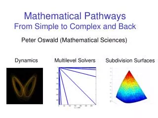
Peter Oswald (Mathematical Sciences). Mathematical Pathways From Simple to Complex and Back. Multilevel Solvers. Subdivision Surfaces. Dynamics. The Complex World of Math(ematicians). ?? Seldomly exercised. Sciences Qualitative and Quantitative Models.

E N D
Peter Oswald (Mathematical Sciences) Mathematical PathwaysFrom Simple to Complex and Back Multilevel Solvers Subdivision Surfaces Dynamics
The Complex World of Math(ematicians) ?? Seldomly exercised Sciences Qualitative and Quantitative Models Mathematics Exact and Abstract Models and Language Ever ChangingReal World Complicated and dirty Full of life Dynamic: Truth is questioned from time to time Clean and beautiful Looks dead (to some) Absolute truth within stated assumptions Success remains interdisciplinary challenge
Complex Numbers Counting: Naturals, Integers 1,2,3,...,n,... ; 0 (zero) ; -1(=1-2),-2,-3,... ; Still: Cannot solve simple quadratic equations such as x + x + 1 = 0 2 Comparing in size: Rationals 1/2, -2/3, ... , p/q, ... y z = x + i y Filling the gaps: Real line Sqrt(2), pi, e, ... i = sqrt(-1) (World of Calculus: Limits, Derivatives, Integrals, ... ) x Complex is also used for sets with structure such as the set of points, line segments, polygons, polyhedra, ... , with incidence relationships (polyhedra have vertices (=points), edges (=line segments), faces (=polygons)) Algebraic Topology
All you need to know about derivatives • Functions of one variable x = x(t) : • The ordinary derivative x‘(t) describes • Instantaneous rate of change of dependent • variable (x) with respect to change in the • independent variable (t) • Geometry: Slope of tangent, x’’(t) related to • curvature • Mechanics: Velocity, x’’(t) is acceleration Functions of several variables u = u(t,x,y,z) : Partial derivatives and differential operators such as gradient or Laplacian
Complex Behavior in Dynamical Systems Transition rule „Next“ State State F Initial state Discrete time: Recursively defined sequences Example: Conway‘s Game of Life ( Cellular Automata) Continuous time: Differential equations such as Selkov model State space 2D 3D Examples: Van der Pol and Lorenz systems
The Game of Life (Conway 1970) State space: Infinite grid of square cells, each cell „live“ or „dead“ State is pattern of marked live cells (or doubly-indexed 0-1 sequence) Transition rules: Look at the 8 neighbors of a cell • A live cell with < 2 live neighbors dies (loneliness) • A live cell with > 3 live neighbors dies (overcrowding) • A live cell with 2 or 3 live neighbors survives • A dead cell with = 3 live neighbors becomes alive (birth process) Initial state: Finite pattern of marked live cells constant pattern period 4 pattern moving period 2 pattern no moving zero pattern n=0 n=1 n=2 n=3 n=4
A Nonlinear Oscillator (Van der Pol 1920-27) |x|>1 damping |x|<1 excitation Periodic force State variable or rewritten as system with state variable (x,y) b=0 b=3 b=30 Limit cycles, quasi-periodic solutions, frequency locking ...
Lorenz system (Lorenz 1963) Smallest system (3 equations) that shows a completely new behavior: Bounded solution trajectories approach a special region (called strange attractor) in a fractal, non-periodic fashion (some kind of deterministic chaos) Rayleigh coefficient: r > 0 Application area: Weather forecasting, reduced model for so-called convection rolls in the lower atmosphere
What have we seen so far? • Complex (dynamic) behavior can be described by simple setups, • both in discrete time (recursive algorithms) and continuous • time (systems of ordinary differential equations). • Similar systems can behave quite differently. In particular, • types of nonlinearity, dimension, parameter changes influence • the behavior. Understanding requires deep Mathematics. • Math and simulation is not all. We don’t know whether our • simple models explain any real mechanism of nature. • This needs good experimentation, data collection and analysis. • Can use the knowledge gained from simple models to analyse • and simulate larger and more complex systems, a common • approach is multi-scaleor hierarchicalmodelling. • Some toy versions of multi-scale algorithms • Solving PDE problems (large small or fine-to-coarse) • Creating shapes (small large or coarse-to-fine) • will be discussed next.
Terrain Triangulation (Multiple Spatial Scales) Courtesy of Prof. Griebel (Scientific Computing, Uni Bonn)
Terrain Triangulation ( Zoom-In Application) Courtesy of Prof. Griebel (Scientific Computing, Uni Bonn)
Multiple Scales in Physical Systems Example: Flow problems Micro/mesoscopic scales: Statistical thermodynamics turbulence particle simulations Macroscopic fields: velocity, pressure, density, temperature,... as functions of space and time (PDEs) Engineering formulas: Drag, peak velocity Example: Integrated circuits Nanoscale: Quantum effects, particle models, MC simulations Macroscopic fields: Electron/hole densities, Potential fields (PDEs) I/O models: Simplified circuit description (ODEs)
Example: Flow simulations Courtesy of Prof. Griebel (Scientific Computing, Uni Bonn) Re Reynolds number f external forces u=(u1,u2,u3) velocity vector p pressure function Most famous system of partial differential equations (PDEs). Describes incompressible fluid motion at constant temperature, and is trusted by 99.999% of scientists (as macroscopic model). PDEs are everywhere (e.g., spatio-temporal effects in bio-systems).
V S V G S S S V S • G S V Example: Electrostatics of ICs q unknown charge density on conductor surface U given electrostatic potential („voltages attached to surface“) Example of an integral equation (IE), also heavily used in engineering simulations. PDEs and IEs of this kind do not possess simple analytic solutions computational methods computer simulations
Unknown functions Vectors of function values on grid • Derivatives Differences • Integrals Sums • PDEs Sparse systems of (linear) equations • IEs Dense systems of (linear) equations Numerical Discretization
Toy Problem: Temperature Distribution T describes stationary temperature field in a square layer (insulated from both sides), with temperature fixed at the edges. Use a (m+1)x(m+1) square grid, each interior grid point carries a discrete temperature value. The PDE (Laplace‘s equation) is discretized by finite differences. This leads altogether to an unknown vector of length n=m*m, and a very sparse, nicely structured linear system of dimension n. x T = 0 (cool surface) T = 20 (Air) T = 20 Corner singularity y T = 200 (hot surface)
Discrete solution m = 40 m = 20
Solving: Gaussian elimination kills The classical solution method (Gaussian elimination) leads to fill-in and becomes impractical for m>100: mxm fill-in block Before elimination After 3 steps After m=6 steps Due to the mxm fill-in block each of the remaining elimination steps Needs roughly ~ m*m = n CPU cycles, i.e., the overall method needs Roughly ~ n*n cycles: Accuracy 0.0001 m~100 ~10 flops (doable but slow) Single precision m~3000 ~10 flops (kills you) 8 14 Need new ideas: Reordering, FFT, Multi-scale (multi-grid) approach
Multiscale Solver: Basic Idea Two ideas: 1) Solve the dicretized problem approximately, not exactly (only within the accuracy of the numerical model which obviously depends on the chosen grid size, i.e., on m) 2) Solve it not only on the given grid but also on a whole hierarchy of coarser grids, and combine cleverly! # flops ~ n Size n Size n/4 Size n/16 Multigrid idea (1960-80) for IEs and PDEs: Fedorenko, Bachvalov, Brandt, Hackbusch,...
Linear Algebra Interpretation badly conditioned nicely conditioned ~ n non-zero entries ~ n log n non-zero entries fast matrix-vector multiplication
Subdivision schemes: Coarse to Fine • Have evolved from the recursive evaluation of spline curves and surfaces into a tool for hierarchical surface generation • Surfaces are created by local topology refinement and geometric rules for inserting new and moving old points in space. They are rendered (displayed) as triangulated surfaces. • Process similar to creating fractal objects • Twist: Result should look smooth (since most shapes consist of smooth pieces)
Dyadic or 2-refinement Insert edge midpoints Quadrisect triangles
Geometric rules (2-subdivision) Interpolating Schemes (old points not moved) Approximating Schemes (old points slightly moved) 3 1 1/2 1/2 (Linear interpolation polyhedra) 1 3 -w 2w -w w(6)=10 1 1 1 1/2 1/2 w(k) 1 1 -w 2w -w (Butterfly scheme, Dyn et al. 1990) (Quartic boxspline, Loop 1987)
Sqrt(3)-refinement (slower topology refinement) Insert face midpoints Create rotated triangulation by joining new and old vertices
How it works (sqrt(3) scheme by Guskov) Step 1 Step 2 Initial configuration Pumpkin? Art? To me: Not so great, artifacts that are not coming from initial shape! Step 6
More Pumpkins: Other Geometric Rules Butterfly: Interpolating Approximating Geometric Rules Slightly different initial configuration
Sqrt(7)-refinement (faster topology refinement) Insert 3 points per triangle (each such point has its “closest” old edge resp. vertex) Connect new points with each other and old vertices in a consistent way (requires orientable triangulation)
Example: Composite Schemes 1. Trivial upsampling:oV 7*oV, nV 0 1/3 3. F2F: 2. V2F: a 1-3a a 1/3 a 1/3 4. F2V: (5. V2V) c/k c/k 1/k 1/k c/k 1-c 1/k 1/k 1/k c/k c/k Repeat 2. – 4.(5.) another (n-1) times
Irregular vertices: Combined scheme for n=2 Double pyramid: k = 3 (not C ) k = 4 (barely C ) Double pyramid: k = 12 (C but too flat) k = 4 (already “treated”) Tetrahedron: k = 3 (not C ) 1 1 1 1
V2V-modification: Tetrahedron before after
V2V-modification: k=3,4 after before
V2V-modification: k=12 before after
Thank you for your attention! Acknowledgements go (in no specific order) to: Wikipedia (Game of Life, Demonstration for Van der Pol equation and Lorenz system, etc.) Matlab (Numerical simulation and visualization support) Prof. Michael Griebel, Dr. Alex Schweitzer, and Group, Institute of Scientific Computing, Uni Bonn (PDE simulations) MS Powerpoint (Hacking it together) Detailed references on request!
Useful URLs: http://www.ibiblio.org/lifepatterns/ (Game of Life implementations) http://www.cmp.caltech.edu/~mcc/Chaos_Course/ (many demos, in particular forced nonlinear oscillator) http://to-campos.planetaclix.pt/fractal/lorenz_eng.html (simulations for Lorenz and Rössler systems) http://wissrech.iam.uni-bonn.de/main/index.html (homepage of Griebel‘s Scientific Computing Group at Uni Bonn, with project descriptions and software for flow problems and many other simulations) http://www.faculty.iu-bremen.de/poswald/teaching/teaching.html (temporary download of today‘s USC talk)