Download
1 / 45
450 likes | 563 Views
So far focused on 3D modeling. Multi-Frame Structure from Motion: Multi-View Stereo. Unknown camera viewpoints. Today. Recognition. Today. Recognition. Recognition problems. What is it? Object detection Who is it? Recognizing identity What are they doing? Activities

E N D
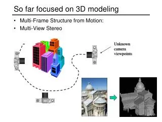
So far focused on 3D modeling • Multi-Frame Structure from Motion: • Multi-View Stereo Unknown camera viewpoints
Today • Recognition
Today • Recognition
Recognition problems • What is it? • Object detection • Who is it? • Recognizing identity • What are they doing? • Activities • All of these are classification problems • Choose one class from a list of possible candidates
How do human do recognition? • We don’t completely know yet • But we have some experimental observations.
Observation 1: The “Margaret Thatcher Illusion”, by Peter Thompson
Observation 1: • http://www.wjh.harvard.edu/~lombrozo/home/illusions/thatcher.html#bottom • Human process up-side-down images seperately The “Margaret Thatcher Illusion”, by Peter Thompson
Observation 2: Kevin Costner Jim Carrey • High frequency information is not enough
Observation 3: • Negative contrast is difficult
Observation 4: • Image Warping is OK
The list goes on • Face Recognition by Humans: Nineteen Results All Computer Vision Researchers Should Know About http://web.mit.edu/bcs/sinha/papers/19results_sinha_etal.pdf
Face detection • How to tell if a face is present?
One simple method: skin detection • Skin pixels have a distinctive range of colors • Corresponds to region(s) in RGB color space • for visualization, only R and G components are shown above skin • Skin classifier • A pixel X = (R,G,B) is skin if it is in the skin region • But how to find this region?
Skin classifier • Given X = (R,G,B): how to determine if it is skin or not? Skin detection • Learn the skin region from examples • Manually label pixels in one or more “training images” as skin or not skin • Plot the training data in RGB space • skin pixels shown in orange, non-skin pixels shown in blue • some skin pixels may be outside the region, non-skin pixels inside. Why?
Skin classification techniques • Skin classifier • Given X = (R,G,B): how to determine if it is skin or not? • Nearest neighbor • find labeled pixel closest to X • choose the label for that pixel • Data modeling • fit a model (curve, surface, or volume) to each class • Probabilistic data modeling • fit a probability model to each class
Probability • Basic probability • X is a random variable • P(X) is the probability that X achieves a certain value • or • Conditional probability: P(X | Y) • probability of X given that we already know Y • called a PDF • probability distribution/density function • a 2D PDF is a surface, 3D PDF is a volume continuous X discrete X
Choose interpretation of highest probability • set X to be a skin pixel if and only if Where do we get and ? Probabilistic skin classification • Now we can model uncertainty • Each pixel has a probability of being skin or not skin • Skin classifier • Given X = (R,G,B): how to determine if it is skin or not?
Approach: fit parametric PDF functions • common choice is rotated Gaussian • center • covariance • orientation, size defined by eigenvecs, eigenvals Learning conditional PDF’s • We can calculate P(R | skin) from a set of training images • It is simply a histogram over the pixels in the training images • each bin Ri contains the proportion of skin pixels with color Ri This doesn’t work as well in higher-dimensional spaces. Why not?
Learning conditional PDF’s • We can calculate P(R | skin) from a set of training images • It is simply a histogram over the pixels in the training images • each bin Ri contains the proportion of skin pixels with color Ri • But this isn’t quite what we want • Why not? How to determine if a pixel is skin? • We want P(skin | R) not P(R | skin) • How can we get it?
what we measure (likelihood) domain knowledge (prior) what we want (posterior) normalization term Bayes rule • In terms of our problem: • The prior: P(skin) • Could use domain knowledge • P(skin) may be larger if we know the image contains a person • for a portrait, P(skin) may be higher for pixels in the center • Could learn the prior from the training set. How? • P(skin) may be proportion of skin pixels in training set
in this case , • maximizing the posterior is equivalent to maximizing the likelihood • if and only if • this is called Maximum Likelihood (ML) estimation Bayesian estimation • Bayesian estimation • Goal is to choose the label (skin or ~skin) that maximizes the posterior • this is called Maximum A Posteriori (MAP) estimation likelihood posterior (unnormalized) = minimize probability of misclassification • Suppose the prior is uniform: P(skin) = P(~skin) = 0.5
H. Schneiderman and T.Kanade General classification • This same procedure applies in more general circumstances • More than two classes • More than one dimension • Example: face detection • Here, X is an image region • dimension = # pixels • each face can be thoughtof as a point in a highdimensional space H. Schneiderman, T. Kanade. "A Statistical Method for 3D Object Detection Applied to Faces and Cars". IEEE Conference on Computer Vision and Pattern Recognition (CVPR 2000) http://www-2.cs.cmu.edu/afs/cs.cmu.edu/user/hws/www/CVPR00.pdf
convert x into v1, v2 coordinates What does the v2 coordinate measure? • distance to line • use it for classification—near 0 for orange pts What does the v1 coordinate measure? • position along line • use it to specify which orange point it is Linear subspaces • Classification can be expensive • Must either search (e.g., nearest neighbors) or store large PDF’s • Suppose the data points are arranged as above • Idea—fit a line, classifier measures distance to line
Dimensionality reduction • How to find v1 and v2 ? • - PCA • Dimensionality reduction • We can represent the orange points with only their v1 coordinates • since v2 coordinates are all essentially 0 • This makes it much cheaper to store and compare points • A bigger deal for higher dimensional problems
Principal component analysis • Suppose each data point is N-dimensional • Same procedure applies: • The eigenvectors of A define a new coordinate system • eigenvector with largest eigenvalue captures the most variation among training vectors x • eigenvector with smallest eigenvalue has least variation • We can compress the data by only using the top few eigenvectors • corresponds to choosing a “linear subspace” • represent points on a line, plane, or “hyper-plane” • these eigenvectors are known as the principal components
= + The space of faces • An image is a point in a high dimensional space • An N x M image is a point in RNM • We can define vectors in this space as we did in the 2D case
Dimensionality reduction • The set of faces is a “subspace” of the set of images • Suppose it is K dimensional • We can find the best subspace using PCA • This is like fitting a “hyper-plane” to the set of faces • spanned by vectors v1, v2, ..., vK • any face
Eigenfaces • PCA extracts the eigenvectors of A • Gives a set of vectors v1, v2, v3, ... • Each one of these vectors is a direction in face space • what do these look like?
Projecting onto the eigenfaces • The eigenfaces v1, ..., vK span the space of faces • A face is converted to eigenface coordinates by
Recognition with eigenfaces • Algorithm • Process the image database (set of images with labels) • Run PCA—compute eigenfaces • Calculate the K coefficients for each image • Given a new image (to be recognized) x, calculate K coefficients • Detect if x is a face • If it is a face, who is it? • Find closest labeled face in database • nearest-neighbor in K-dimensional space
i = K NM Choosing the dimension K • How many eigenfaces to use? • Look at the decay of the eigenvalues • the eigenvalue tells you the amount of variance “in the direction” of that eigenface • ignore eigenfaces with low variance eigenvalues
Issues: dimensionality reduction • What if your space isn’t flat? • PCA may not help Nonlinear methodsLLE, MDS, etc.
Issues: data modeling • Generative methods • model the “shape” of each class • histograms, PCA, • mixtures of Gaussians • ... • Discriminative methods • model boundaries between classes • perceptrons, neural networks • support vector machines (SVM’s)
Generative vs. Discriminative Generative Approachmodel individual classes, priors Discriminative Approachmodel posterior directly from Chris Bishop
Issues: speed • Case study: Viola Jones face detector • Exploits three key strategies: • simple, super-efficient features • image pyramids • pruning (cascaded classifiers)
{ { +1 if ft(x) > qt -1 otherwise face, if Y(x) > 0 non-face, otherwise Detection = ht(x) = Viola/Jones: features “Rectangle filters” Differences between sums of pixels in adjacent rectangles Unique Features Y(x)=∑αtht(x) Select 200 by Adaboost Robust Realtime Face Dection, IJCV 2004, Viola and Jonce
Integral Image (aka. summed area table) • Define the Integral Image • Any rectangular sum can be computed in constant time: • Rectangle features can be computed as differences between rectangles
Larger Scale Smallest Scale Viola/Jones: handling scale 50,000 Locations/Scales
Cascaded Classifier • first classifier: 100% detection, 50% false positives. • second classifier: 100% detection, 40% false positives • (20% cumulative) • using data from previous stage. • third classifier: 100% detection,10% false positive rate • (2% cumulative) • Put cheaper classifiers up front 50% 20% 2% IMAGE SUB-WINDOW 5 Features 20 Features FACE 1 Feature F F F NON-FACE NON-FACE NON-FACE
Viola/Jones results: Run-time: 15fps (384x288 pixel image on a 700 Mhz Pentium III)
Application Smart cameras: auto focus, red eye removal, auto color correction
Application Lexus LS600 Driver Monitor System