Download
1 / 21
210 likes | 394 Views
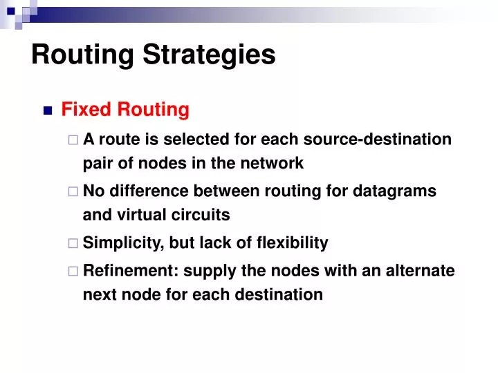
Routing Strategies. Fixed Routing A route is selected for each source-destination pair of nodes in the network No difference between routing for datagrams and virtual circuits Simplicity, but lack of flexibility Refinement: supply the nodes with an alternate next node for each destination.

E N D
Routing Strategies • Fixed Routing • A route is selected for each source-destination pair of nodes in the network • No difference between routing for datagrams and virtual circuits • Simplicity, but lack of flexibility • Refinement: supply the nodes with an alternate next node for each destination
Routing Strategies (cont) • Flooding • A packet is sent by a source node to every one of its neighbors • At each node, an incoming packet is retx on all outgoing link except for the link on which it arrived • Hop count field deals with duplicate copies of a pkt • Properties • All possible routes btw source and destination are tried • At least one copy of the packet to arrive at the destination will have a minimum-hop route • All nodes connected to the source node are visited
Routing Strategies (cont) • Random Routing • Selects only one outgoing path for retx of an incoming packet • Assign a probability to each outgoing link and to select the link based on that probability • Adaptive Routing • Routing decisions that are made change as conditions on the network change • Failure • Congestion
Routing Strategies (cont) • Adaptive Routing • State of the network must be exchanged among the nodes • Routing decision is more complex • Introduces traffic of state information to the network • Reacting too quickly will cause congestion-producing oscillation • If it reacts too slowly, the strategy will be irrelevant
Shortest Path Algorithm • Dijkstra’s Algorithm • Bellman-Ford Algorithm 8 5 3 3 5 2 6 6 2 8 3 3 2 1 4 1 2 3 1 2 1 1 7 4 5 1
Reduced graph 5 3 3 5 2 6 2 1 1 2 3 2 1 4 5 1
Dijkstra’s Algorithm 2 3 2 3 D2 = 2 D3 = 4 D2 = 2 D3 = 5 1 1 6 6 4 5 4 5 D4 = 1 D4 = 1 D5 = 2 M = { 1, 4 } M = { 1 } D3 = 3 2 3 2 3 D2 = 2 D3 = 4 D2 = 2 1 1 6 6 D6 = 4 4 5 4 5 D4 = 1 D5 = 2 D4 = 1 D5 = 2 M = { 1, 2, 4 } M = { 1, 2, 4, 5 }
Dijkstra’s Algorithm (cont) Node D M 2 3 4 5 6 ¥ ¥ 1 2 5 1 1, 4 ¥ 2 4 1 2 ¥ 1, 4, 2 2 4 1 2 1, 4, 2, 5 2 3 1 2 4 1, 4, 2, 5, 3 2 3 1 2 4 1, 4, 2, 5, 3, 6 2 3 1 2 4
Dijkstra’s Algorithm (cont) • w(i, j) = link cost, L(n) = path cost from node s to n • 1. [Initialization] • T = {s} • L(n) = w (s, n) for n ≠ s • 2. [Get next node] • Find x Ï T such that L(x) = min L(j) • Add x to T • 3. [Update Least-Cost Paths] • L(n) = min [ L(n), L(x)+w(x, n) ] for all n Ï T • Go to step 2 jÏT
Bellman-Ford Algorithm D(2)3 = 4 2 3 2 3 D(1)2 = 2 D(1)3 = 5 D(2)2 = 2 1 1 6 6 D(2)6 = 10 4 5 4 5 D(1)4 = 1 D(2)4 = 1 D(2)5 = 2 h = 1 h = 2 D(3)3 = 3 2 3 D(3)2 = 2 1 6 D(3)6 = 4 4 5 D(3)4 = 1 D(3)5 = 2 h = 3
Bellman-Ford Algorithm (cont) Node D h 2 3 4 5 6 ¥ ¥ ¥ ¥ ¥ 0 Source = 1 ¥ ¥ 1 2 5 1 2 2 4 1 2 10 3 2 3 1 2 4 4 2 3 1 2 4
link j s n <= h links Bellman-Ford Algorithm (cont) • Lh(n) = path cost from s to n w/ no more than h links • 1. [Initialization] • L0(n) = ∞, for all n ≠ s • Lh(s) = 0, for all h • 2. [Update] • For each successive h ≥ 0 • For each n ≠ s, compute • Lh+1(n) = min [ Lh(j) + w(j, n) ] j
Comparisons L(n) = min [ L(n), L(x)+w(x, n) ] Lh(x, D) x … …… S D S D x x Dijkstra’s (Link State) Bellman-Ford (Distance Vector)
Routing in ARPANET • First generation(RIP), 1969 • Adaptive Routing is adopted • Use Bellman-Ford algorithm • Estimated link delay is simply the queue length for that link • Every 128ms, each node exchanges its delay vector(routing table) with all its neighbors • Information about a change in network condition would gradually ripple through the network
j k i Routing in ARPANET (cont) • Each node i maintains • di j = current estimate of min delay from i to j • si j = next node in the current min-delay route from i to j • Node k updates its vectors as follows • dk j = Min [ lk i + di j ] i Î A • sk j = i using i that minimizes the expression abovewhereA = set of neighbor nodes for klk i = current estimate of delay from k to i
Routing in ARPANET (cont) • Major shortcomings of RIP • It did not consider line speed, merely queue length. Higher capacity links were not given the favored status • Queue length is an artificial measure of delay • The algorithm was not very accurate. It responded slowly to congestion and delay increases.
Routing in ARPANET (cont) • Second generation, 1979 • OSPF: Open Shortest Path First protocol • Link-state routing protocol • The delay is measured directly • Every 10 seconds, the node computes the average delay on each outgoing link • Information of changes in delay is sent to all others nodes using flooding • Using Dijkstra’s algorithm
Routing in ARPANET (cont) • Third generation, 1987 • Problem • The correlation between the reported values (delay) and those actually experienced after rerouting • Conclusion • Under heavy load, the goal of routing should be to give the average route a good path instead of attempting to give all routes the best path • Solution • Also consider the average utilization of links • Revisedcost function: delay-based metric under light loads, capacity-based metric under heavy loads
Calculate Link Costs • Measure the avg. delay over the last 10 sec • Using the single-server queuing model, the measured delay is transformed into an estimate of link utilization • Average the link utilization with the previous estimate of utilization • The link cost is set as a function of average utilization
0.0 0.1 0.2 0.3 0.4 0.5 0.6 0.7 0.8 0.9 1.0 ARPANET Delay Metrics (3rd) Theoreticalqueueing delay 5 4 Delay (hops) 3 Metric forsatellite link 2 Metric forterrestrial link 1 0 Estimated utilization