Download
1 / 42
420 likes | 615 Views
Routing. Outline Algorithms Scalability. Overview. Forwarding vs Routing forwarding: to select an output port based on destination address and routing table routing: process by which routing table is built Network as a Graph Problem: Find lowest cost path between two nodes Factors

E N D
Routing Outline Algorithms Scalability CS 461
Overview • Forwarding vs Routing • forwarding: to select an output port based on destination address and routing table • routing: process by which routing table is built • Network as a Graph • Problem: Find lowest cost path between two nodes • Factors • static: topology • dynamic: load CS 461
Overview • A routing domain: an internet work in which all the routers are under the same administrative control. • Intradomain routing protocol (interior gateway protocols) • Interdomain routing protocol (exterior gateway protocols) CS 461
Distance Vector • Each node maintains a set of triples • (Destination, Cost, NextHop) • Directly connected neighbors exchange updates • periodically (on the order of several seconds) • whenever table changes (called triggered update) • Each update is a list of pairs: • (Destination, Cost) • Update local table if receive a “better” route • smaller cost • came from next-hop • Refresh existing routes; delete if they time out CS 461
Example Destination Cost NextHop A 1 A C 1 C D 2 C E 2 A F 2 A G 3 A Routing Table for B CS 461
Routing Loops • Example 1 • F detects that link to G has failed • F sets distance to G to infinity and sends update t o A • A sets distance to G to infinity since it uses F to reach G • A receives periodic update from C with 2-hop path to G • A sets distance to G to 3 and sends update to F • F decides it can reach G in 4 hops via A • Example 2 • link from A to E fails • A advertises distance of infinity to E • B and C advertise a distance of 2 to E • B decides it can reach E in 3 hops; advertises this to A • A decides it can read E in 4 hops; advertises this to C • C decides that it can reach E in 5 hops… CS 461
(2,A) 4 B (3,B) B 3 (1,E) 3 C C A A (4,C) 4 E E D D (2,A) 4 (3,F) F F 3 G G (2,A) B (3,B) (3,B) C A (4,C) E D (2,A) (3,F) F G Count to infinity problem 4 B 5 5 C A 4 E D 4 F 5 G CS 461
8 6 6 B B B 7 7 5 7 5 7 C C C A A A 8 6 6 E E E D D D D D D 6 8 6 F F F 7 5 7 G G G Count to infinity problem (cont.) CS 461
Split horizon with poison reverse • If in the routing table of a neighbor Y of node X, the next hop entry for destination Z is X, Y informs X that its distance to Z is infinite. CS 461
(,-) (2,A) (2,A) B B B (,-) (3,B) (3,B) (,E) (1,E) (,E) C C C A A A (4,C) (4,C) (4,C) E E E D D D (2,A) (2,A) (,-) (3,F) (,-) (3,F) F F F G G G (,-) B (3,B) (,E) C A (4,C) E D (,-) (3,F) F G CS 461
(,-) (3,C) (2,A) (2,A) B B B B (2,A) (3,B) (2,A) (,-) (4,B) (,E) (,E) (1,E) C C C C A A A A (3,C) (3,C) (4,C) (3,C) E E E E D D D D (,-) (,-) (2,A) (2,A) (4,D) (3,F) (3,F) (3,F) F F F F G G G G Split horizon with poison reverse cannot solve the count-to-infinity problem CS 461
(6,C) (7,A) (8,A) (,-) B B B B (8,A) (,-) (5,A) (7,A) (7,F) (6,F) (,-) (,-) C C C C A A A A (6,C) (8,C) (,-) (,-) E E E E D D D D (,-) (5,G) (6,G) (,-) (,-) (,-) (5,D) F F F F G G G G Split horizon with poison reverse cannot solve the count-to-infinity problem (,-) CS 461
Loop-Breaking Heuristics • Set infinity to 16 • Split horizon • Split horizon with poison reverse CS 461
Link State • Strategy • send to all nodes (not just neighbors) information about directly connected links (not entire routing table) • Link State Packet (LSP) • id of the node that created the LSP • cost of link to each directly connected neighbor • sequence number (SEQNO) • time-to-live (TTL) for this packet CS 461
Link State (cont) • Reliable flooding • store most recent LSP from each node • forward LSP to all nodes but one that sent it • generate new LSP periodically • increment SEQNO • start SEQNO at 0 when reboot • decrement TTL of each stored LSP • discard when TTL=0 CS 461
Route Calculation • Dijkstra’s shortest path algorithm • Let • N denotes set of nodes in the graph • l (i, j) denotes non-negative cost (weight) for edge (i, j) • s denotes this node • M denotes the set of nodes incorporated so far • C(n) denotes cost of the path from s to node n M = {s} for each n in N - {s} C(n) = l(s, n) while (N != M) M = M union {w} such that C(w) is the minimum for all w in (N - M) for each n in (N - M) C(n) = MIN(C(n), C (w) + l(w, n )) CS 461
Metrics • Original ARPANET metric • measures number of packets queued on each link • took neither latency or bandwidth into consideration • New ARPANET metric • stamp each incoming packet with its arrival time (AT) • record departure time (DT) • when link-level ACK arrives, compute Delay = (DT - AT) + Transmit + Latency • if timeout, reset DT to departure time for retransmission • link cost = average delay over some time period • Fine Tuning • compressed dynamic range • replaced Delay with link utilization CS 461
How to Make Routing Scale • Flat versus Hierarchical Addresses • Inefficient use of Hierarchical Address Space • class C with 2 hosts (2/255 = 0.78% efficient) • class B with 256 hosts (256/65535 = 0.39% efficient) • Still Too Many Networks • routing tables do not scale • route propagation protocols do not scale CS 461
Internet Structure Recent Past NSFNET backbone Stanford ISU BARRNET MidNet ■ ■ ■ regional Westnet regional regional Berkeley PARC UNL KU UNM NCAR UA CS 461
Large corporation “Consumer” ISP Peering point Backbone service provider Peering point “Consumer” ISP “Consumer” ISP Large corporation Small corporation Internet Structure Today CS 461
Subnetting • Add another level to address/routing hierarchy: subnet • Subnet masks define variable partition of host part • Subnets visible only within site CS 461
Subnet Example Forwarding table at router R1 Subnet Number Subnet Mask Next Hop 128.96.34.0 255.255.255.128 interface 0 128.96.34.128 255.255.255.128 interface 1 128.96.33.0 255.255.255.0 R2 CS 461
Forwarding Algorithm D = destination IP address for each entry (SubnetNum, SubnetMask, NextHop) D1 = SubnetMask & D if D1 = SubnetNum if NextHop is an interface deliver datagram directly to D else deliver datagram to NextHop • Use a default router if nothing matches • Not necessary for all 1s in subnet mask to be contiguous • Can put multiple subnets on one physical network • Subnets not visible from the rest of the Internet CS 461
Supernetting • Assign block of contiguous network numbers to nearby networks • Called CIDR: Classless Inter-Domain Routing • Represent blocks with a single pair (first_network_address, count) • Restrict block sizes to powers of 2 • Use a bit mask (CIDR mask) to identify block size • All routers must understand CIDR addressing CS 461
Route Propagation • Know a smarter router • hosts know local router • local routers know site routers • site routers know core router • core routers know everything • Autonomous System (AS) • corresponds to an administrative domain • examples: University, company, backbone network • assign each AS a 16-bit number • Two-level route propagation hierarchy • interior gateway protocol (each AS selects its own) • exterior gateway protocol (Internet-wide standard) CS 461
Popular Interior Gateway Protocols • RIP: Route Information Protocol • developed for XNS • distributed with Unix • distance-vector algorithm • based on hop-count • OSPF: Open Shortest Path First • recent Internet standard • uses link-state algorithm • supports load balancing • supports authentication CS 461
EGP: Exterior Gateway Protocol • Overview • designed for tree-structured Internet • concerned with reachability, not optimal routes • Protocol messages • neighbor acquisition: one router requests that another be its peer; peers exchange reachability information • neighbor reachability: one router periodically tests if the another is still reachable; exchange HELLO/ACK messages; uses a k-out-of-n rule • routing updates: peers periodically exchange their routing tables (distance-vector) CS 461
BGP-4: Border Gateway Protocol • AS Types • stub AS: has a single connection to one other AS • carries local traffic only • multihomed AS: has connections to more than one AS • refuses to carry transit traffic • transit AS: has connections to more than one AS • carries both transit and local traffic • Each AS has: • one or more border routers • one BGP speaker that advertises: • local networks • other reachable networks (transit AS only) • gives path information CS 461
BGP Example • Speaker for AS2 advertises reachability to P and Q • network 128.96, 192.4.153, 192.4.32, and 192.4.3, can be reached directly from AS2 • Speaker for backbone advertises • networks 128.96, 192.4.153, 192.4.32, and 192.4.3 can be reached along the path (AS1, AS2). • Speaker can cancel previously advertised paths CS 461
IP Version 6 • Features • 128-bit addresses (classless) • multicast • real-time service • authentication and security • autoconfiguration • end-to-end fragmentation • protocol extensions • Header • 40-byte “base” header • extension headers (fixed order, mostly fixed length) • fragmentation • source routing • authentication and security • other options CS 461
Address Notation: X:X:X:X:X:X:X:X • Where X is a hexadecimal representation of a 16-bit piece of the address. • Example: 47CD:1234:4422:AC02:0022:1234:A456:0124 • 47CD:0000:0000:0000:0000:0000:A456:0124 • 47CD::A456:0124 • Reserved Addresses: prefix 0000 0000 • IPv4-comatible IPv6 address • 0000:0000:…:0000:0000:128.96.33.81(IPv4 address) • ::128.96.33.81 • IPv4-mapped IPv6 address (for node that is only capable of understanding IPv4) • 0000:0000:…:FFFF:128.96.33.81 • ::FFFF:128.96.33.81 CS 461
Aggregatable Global Unicast Addresses: prefix 001 • Use CIDR prefix addressing • Link local use addresses: prefix 1111 1110 10 • Site local use addresses: prefix 1111 1110 11 • - Global uniqueness of the address need no be an issue • - Autoconfiguration (plug and play) • Use link local use addresses • 1111 1110 10 0…0 + 48-bit Ethernet address • 0’s • Router advertise the subnet prefix CS 461
Multicast Addresses: prefix 1111 1111 • Anycast Addresses: use regular unicast addresses • -To deliver a packet to one of a group of addresses, usually the nearest one • -Routing support to mobile hosts • Other Issues: • -Secutiry • -QoS CS 461
IPv4 IPv6 capable IPv6 capable • Transition from IPv4 to IPv6 • Some IPv6 capable nodes, Some hosts and routers that only understand IPv4 • Two major mechanisms: • 1. Dual-stack operation • IPv6 nodes: use version field (to decide which stack should process the incoming packets) • 2. Tunneling CS 461