Download

1 / 36
360 likes | 369 Views
Probability Density Functions of Liquid Water Path and Total Water Content of Marine Boundary Layer Clouds. Hideaki Kawai Japan Meteorological Agency Joao Teixeira Jet Propulsion Laboratory, Caltech. Today’s Talk. 1. Data

E N D
Probability Density Functions of Liquid Water Path and Total Water Content ofMarine Boundary Layer Clouds Hideaki Kawai Japan Meteorological Agency Joao Teixeira Jet Propulsion Laboratory, Caltech
Today’s Talk 1. Data 2. Relationships between PDFs of LWP and PDFs of total water content 3. Impact of inhomogeneity on precipitation and radiation processes 4. PDFs for various types of marine boundary layer
1. Data • Data : GOES visible channel data (0.55-0.75µm) • * spatial resolution : 1km mesh • * temporal resolution : less than 30 minutes • Location : GPCI line, 20S line, 88W line • (Each line consists of 8 locations) • Area size : 200km x 200km • Period : 1999-2001 (Jan, Apr, Jul, Oct) • Number of used snapshots : • ~ 100,000 • (3 (lines) x 8 (locations) x 3 (years) x 4 (months) • x 30 (days/month) x 10-20 (times/day))
GPCI line 88W line 20S line EPIC Buoy
Homogeneity : Skewness : S Kurtosis : K Wood and Hartmann (2006)
Relationship among PDFs of total water content, liquid water content and liquid water path Assumptions (1) Average of Total Water Content is constant in the mixed layer. (2) PDF of total water content is the same through the mixed layer. (3) Saturation specific humidity decreases linearly upward. (4) Spatial fluctuation of total water content is vertically coherent. (Structure of overlap of PDF is correlated completely.
Under the assumptions, what should the relationship between PDFs of Liquid Water Path and PDFs of total water content be? Liquid Water Path : depth of cloud, : just below the cloud top using the substitution PDF of (1) As a result, this equation is mathematically equivalent to the equation of PDFs of cloud depth and PDFs of LWP by Considine et al (1997).
Examples of PDFs of and corresponding PDFs of PDF of total water content Uniform Triangular Gaussian PDF of liquid water content (at the cloud top) corresponding PDF of liquid water path ( X and Y axes are normalized so that the integral of the PDF =1 and σ of the PDF=1. )
Relationship between cloud amount and skewness of LWP PDFs Skewness Cloud Amount Points : Observation data ● : median ○ : 25th & 75th percentile values All the original data (~100,000 snapshots ) are used for this statistics. Lines : Theoretical Curves Two lines correspond to two mimicked detection limits (10% or 20% of average liquid water path).
3. Impact of inhomogeneity on precipitation process and radiation process
Correction ratio for autoconversion rate Often used equation of autoconversion rate : LWC Calculation used usually in GCMs Want to know this ratio! More appropriate calculation Correction ratio for autoconversion rate
Correction ratio for Autoconversion rate Correction Ratio Cloud Amount[%] PDF of total water content is assumed to be Gaussian.
Reduction factor for LWP used in radiation process Want to know this factor! Effective Thickness Approach (ETA) To get the factor Effective LWP : a function to convert reflectance to LWP
Reduction factor used in radiation processes Reduction Factor Cloud Amount[%] PDF of total water content is assumed to be Gaussian and corresponding PDF of LWP is derived analytically.
Relationship between cloud amount and skewness of LWP PDFs Skewness Four ABL types categorized using h*850-h1000 Cloud Amount [%]
Summary 0. Subgrid-scale variability of marine boundary layer cloud LWPs is investigated using GOES visible channel data. 1. Generally speaking, Gaussian function seems to represent PDFs of total water content well under the set of our assumptions. 2. Effect of inhomogeneity of cloud water on autoconversion rate and shortwave reflectance are deduced as a function of cloud amount. 3. When the ABL is strongly or moderately stable, PDFs of total water content is triangular or Gaussian. On the other hand, when the ABL is unstable, the shape of the PDFs is almost unique with low homogeneity and high skewness & kurtosis.
The End Thank you!
Processing • Count Data -> Radiance • post launch calibration, solar zenith angle calibration • Radiance -> Reflectance • Reflectance -> Liquid water path • Using the relationship by Han et al. (1998) (re: MODIS) • Elimination of Middle & High Clouds • Using infrared channel (IR1, 10.2-11.2µm) • * Criterion : Tbb<Tsea-Toffset-15 -> M.-CL or H.-CL • * More than 1% -> The snapshot is not used. • Cloud Threshold • * threshold albedo = 0.13 (LWP=5[g/m2])
Comparison between LWP from GOES and EPIC LWP 6 days data is used
Comparison between Homogeneity/Skewness from GOES and MODIS Homo. (MODIS) Homogeneity Homo. (GOES) Skew. (MODIS) Skewness Skew. (GOES)
GPCI line Larger γ, smaller S and K toward sea coast. Largest γ, smallest S and K are in NH summer. Spatial variation is larger than seasonal variation. Along SH line, results are similar. Each dot : median of 30 (days/month) x 3 (years) daily-averaged data Bars : 90% confidence intervals from bootstrap method
20S line Largest γ, smallest S and K are in SH winter and spring.
88W line Largest γ, smallest S and K are in SH winter and spring. Seasonal variation is larger than spatial variation.
Used meteorological data : ERA40 • Parameters examined sensible heat flux, latent heat flux, Psea, U10m, V10m, 10m wind speed, temperature advection near surface, T2m, lifting condensation level, ω700, ω850, U850, V850, Wind shear (850-1000), RH850, RH925, RH1000, θ700−θ1000, θv700−θv1000, h*700−h1000, EIS (Wood & Bretherton 2006), θ775−θ1000, θv775−θv1000, h*775−h1000, θ850−θ1000, θv850−θv1000, h*850−h1000, (h850−h1000) − k·L· (q850−q1000) (k=0.70, 0.53, 0.23), h850−h1000, Buoyancy of plume: Tplume(850<-1000)−T850, Tv plume(850<-1000)−Tv850 Δθe − k·(L/Cp)· Δqt • Used Metric Spearman’s rank correlation, Kendall’s rank correlation, Pearson’s correlation • Above Metrics are calculated for monthly-based data, daily data, daily anomaly data to each month data.
As an example, if CGLMSE (k=0.70) is plotted in X axis… Location closest to the land Each color consists of 8 locations x 4 seasons.
(The case that PDFs of LWP themselves are conventional functions) These conventional functions seem not to be able to represent PDFs of Liquid Water Path...
Relationship between cloud amount and homogeneity of LWP PDFs Homogeneity Cloud Amount Points : Observation data ● : median ○ : 25th & 75th percentile values All the original data (~100,000 snapshots ) are used for this statistics. Lines : Theoretical Curves Two lines correspond to two mimicked detection limits (10% or 20% of average liquid water path).
Relationship between cloud amount and skewness/kurtosis of LWP PDFs Skewness Kurtosis Cloud Amount Cloud Amount When PDFs of total water content are assumed to be Gaussian, the corresponded functions derived using the conceptual model are able to represent the observed relationship between cloud amount and statistical properties of PDFs of Liquid Water Path relatively well.
Relationship between cloud amount and skewness/kurtosis of LWP PDFs Skewness Kurtosis Cloud Amount [%] Cloud Amount [%] When ABL is strongly stable, the PDFs of total water content tend to be similar to Triangular distribution. When ABL is unstable, the PDFs have a unique shape with low homogeneity, high skewness and high kurtosis regardless of the cloud amount.
Effect of inhomogeneity on conversion of cloud water to precipitation Production of Precipitation
Effect of inhomogeneity on shortwave reflectance Shortwave Reflectance : Optical Thickness
Four ABL types categorized using h*850-h1000 US WS MS SS US WS MS SS US : Unstable , WS : Weakly Stable MS : Moderately Stable , SS : Strongly Stable