Download
1 / 76
810 likes | 1.09k Views
Implementing Cognitive Radio. How does a radio become cognitive?. Presentation Overview. Architectural Approaches Observing the Environment Autonomous Sensing Collaborative Sensing Radio Environment Maps and Observation Databases Recognizing Patterns Neural Nets Hidden Markov Models

E N D
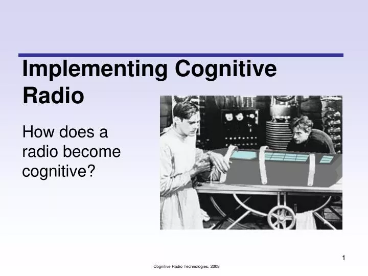
Implementing Cognitive Radio How does a radio become cognitive? Cognitive Radio Technologies, 2008
Presentation Overview • Architectural Approaches • Observing the Environment • Autonomous Sensing • Collaborative Sensing • Radio Environment Maps and Observation Databases • Recognizing Patterns • Neural Nets • Hidden Markov Models • Making Decisions • Common Heuristic Approaches • Case-based Reasoning • Representing Information • A Case Study Cognitive Radio Technologies, 2008
Architectural Overview What are the components of a cognitive radio and how do they relate to each other? Cognitive Radio Technologies, 2008
Strong Artificial Intelligence • Concept: Make a machine aware (conscious) of its environment and self aware Cognitive Radio Technologies, 2008 (probably a good thing) • A complete failure
Weak Artificial Intelligence • Concept: Develop powerful (but limited) algorithms that intelligently respond to sensory stimuli • Applications • Machine Translation • Voice Recognition • Intrusion Detection • Computer Vision • Music Composition Cognitive Radio Technologies, 2008
Weak cognitive radio Radio’s adaptations determined by hard coded algorithms and informed by observations Many may not consider this to be cognitive (see discussion related to Fig 6 in 1900.1 draft) Strong cognitive radio Radio’s adaptations determined by conscious reasoning Closest approximation is the ontology reasoning cognitive radios Implementation Classes • In general, strong cognitive radios have potential to achieve both much better and much worse behavior in a network. Cognitive Radio Technologies, 2008
Weak/Procedural Cognitive Radios • Radio’s adaptations determined by hard coded algorithms and informed by observations • Many may not consider this to be cognitive (see discussion related to Fig 6 in 1900.1 draft) • A function of the fuzzy definition • Implementations: • CWT Genetic Algorithm Radio • MPRG Neural Net Radio • Multi-dimensional hill climbing DoD LTS (Clancy) • Grambling Genetic Algorithm (Grambling) • Simulated Annealing/GA (Twente University) • Existing RRM Algorithms? Cognitive Radio Technologies, 2008
Strong Cognitive Radios • Radio’s adaptations determined by some reasoning engine which is guided by its ontological knowledge base (which is informed by observations) • Proposed Implementations: • CR One Model based reasoning (Mitola) • Prolog reasoning engine (Kokar) • Policy reasoning (DARPA xG) Cognitive Radio Technologies, 2008
Decision, Action DFS in 802.16h Service in function Channel Availability Check on next channel Choose Different Channel Observation • Drafts of 802.16h defined a generic DFS algorithm which implements observation, decision, action, and learning processes • Very simple implementation Available? No Observation Yes In service monitoring of operating channel Decision, Action No Detection? Select and change to new available channel in a defined time with a max. transmission time Yes Stop Transmission Learning Start Channel Exclusion timer Log of Channel Availability Channel unavailable for Channel Exclusion time Yes Available? No Background In service monitoring (on non-operational channels) Cognitive Radio Technologies, 2008 Modified from Figure h1 IEEE 802.16h-06/010 Draft IEEE Standard for Local and metropolitan area networks Part 16: Air Interface for Fixed Broadband Wireless Access Systems Amendment for Improved Coexistence Mechanisms for License-Exempt Operation, 2006-03-29
Example Architecture from CWT Observation Orientation Action Decision Learning Cognitive Radio Technologies, 2008 Models
Architecture Summary • Two basic approaches • Implement a specific algorithm or specific collection of algorithms which provide the cognitive capabilities • Specific Algorithms • Implement a framework which permits algorithms to be changed based on needs • Cognitive engine • Both implement following processes • Observation, Decision, Action • Either approach could implement • Learning, Orientation • Negotiation, policy engines, models • Process boundaries may blur based on the implementation • Signal classification could be orientation or observation • Some processes are very complementary • Orientation and learning • Some processes make most intuitive sense with specific instantiations • Learning and case-based-reasoning Cognitive Radio Technologies, 2008
Observations How does the radio find out about its environment? Cognitive Radio Technologies, 2008
Information is about How the cognitive radio gets the information? Other opportunities to get information Environment (physical quantities, position, situations) • Measures temperature, light level, humidity, … • Receives GPS signals to determine position • Parses short-range wireless broadcasts in buildings or urban areas for mapped environment • Observes the network for e.g. weather forecast, reported traffic jams, …etc. Spectrum (communication opportunities) • Passively "listens" to the spectrum • Performs channel quality estimation • Spectrum information is provided by the network • Spectrum information is shared by other cognitive radios User • Observes user's applications, incoming/ outgoing data streams • Performs speech analysis The Cognitive Radio and its Environment Cognitive Radio Technologies, 2008
Signal Detection • Optimal technique is matched filter • While sometimes useful, matched filter may not be practical for cognitive radio applications as the signals may not be known • Frequency domain analysis often required • Periodogram • Fourier transform of autocorrelation function of received signal • More commonly implemented as magnitude squared of FFT of signal Cognitive Radio Technologies, 2008
Comments on Periodogram • Spectral leaking can mask weak signals • Resolution a function of number of data points • Significant variance in samples • Can be improved by averaging, e.g., Bartlett, Welch • Less resolution for the complexity • Significant bias in estimations (due to finite length) • Can be improved by windowing autocorrelation, e.g., Blackman-Tukey Quality Factor Cognitive Radio Technologies, 2008
Other Detection Techniques • Nonparametric • Goertzel – evaluates Fourier Transform for a small band of frequencies • Parametric Approaches • Need some general characterization (perhaps as general as sum of sinusoids) • Yule-Walker (Autoregressive) • Burg (Autoregressive) • Eigenanalysis • Pisarenko Harmonic Decomposition • MUSIC • ESPRIT Cognitive Radio Technologies, 2008
Sub noise floor Detection • Detecting narrowband signals with negative SNRs is actually easy and can be performed with preceding techniques • Problem arises when signal PSD is close to or below noise floor • Pointers to techniques: • (white noise) C. L. Nikias and J. M. Mendel, “Signal processing with higher-order spectrum,” Signal Processing, July 1993. • (Works with colored noise and time-varying frequencies) K. Hock, “Narrowband Weak Signal Detection by Higher Order Spectrum,” Signal Processing, April 1996 • C.T. Zhou, C. Ting, “Detection of weak signals hidden beneath the noise floor with a modified principal components analysis,” AS-SPCC 2000, pp. 236-240. Cognitive Radio Technologies, 2008
Signal Classification • Detection and frequency identification alone is often insufficient as different policies are applied to different signals • Radar vs 802.11 in 802.11h,y • TV vs 802.22 • However, would prefer to not have to implement processing to recover every possible signal • Spectral Correlation permits feature extraction for classification Cognitive Radio Technologies, 2008
Cyclic Autocorrelation • Cyclic Autocorrelation • Quicky terminology: • Purely Stationary • Purely Cyclostationary • Exhibiting Cyclostationarity • Meaning: periods of cyclostationarity correspond to: • Carrier frequencies, pulse rates, spreading code repetition rates, frame rates • Classify by periods exhibited in R Cognitive Radio Technologies, 2008
Spectral Correlation • Estimation of Spectral Correlation Density (SCD) • For =0, above is periodogram and in the limit the PSD • SCD is equivalent to Fourier Transform of Cyclic Autocorrelation Cognitive Radio Technologies, 2008
Spectral Coherence Function • Spectral Coherence Function • Normalized, i.e., • Terminology: • = cycle frequency • f = spectrum frequency • Utility: Peaks of C correspond to the underlying periodicities of the signal that may be obscured in the PSD • Like periodogram, variance is reduced by averaging Cognitive Radio Technologies, 2008
Practical Implementation of Spectral Coherence Function From Figure 4.1 in I. Akbar, “Statistical Analysis of Wireless Systems Using Markov Models,” PhD Dissertation, Virginia Tech, January 2007 Cognitive Radio Technologies, 2008
Example Magnitude Plots BPSK DSB-SC AM FSK MSK Cognitive Radio Technologies, 2008
- Profile • -profile of SCF • Reduces data set size, but captures most periodicities BPSK DSB-SC AM MSK FSK Cognitive Radio Technologies, 2008
Combination of Signals MSK BPSK BPSK + MSK Cognitive Radio Technologies, 2008
Main signature remains BPSK with SNR=9dB BPSK with SNR=-9dB Impact of Signal Strength Cognitive Radio Technologies, 2008
Resolution BPSK 200x200 • High resolution may be needed to capture feature space • High computational burden • Lower resolution possible if there are expected features • Legacy radios should be predictable • CR may not be predictable • Also implies an LPI strategy BPSK 100x100 AM Cognitive Radio Technologies, 2008 Plots from A. Fehske, J. Gaeddert, J. Reed, “A new approach to signal classification using spectral correlation and neural networks,”DySPAN 05, pp. 144-150.
Additional comments on Spectral Correlation • Even though PSDs may overlap, spectral correlation functions for many signals are quite distinct, e.g., BPSK, QPSK, AM, PAM • Uncorrelated noise is theoretically zeroed in the SCF • Technique for subnoise floor detection • Permits extraction of information in addition to classification • Phase, frequency, timing • Higher order techniques sometimes required • Some signals will not be very distinct, e.g., QPSK, QAM, PSK • Some signals do not exhibit requisite second order periodicity Cognitive Radio Technologies, 2008
Collaborative Observation • Possible to combine estimations • Reduces variance, improves PD vs PFA • Should be able to improve resolution • Proposed for use in 802.22 • Partition cell into disjoint regions • CPE feeds back what it finds • Number of incumbents • Occupied bands Cognitive Radio Technologies, 2008 Source: IEEE 802.22-06/0048r0
More Expansive Collaboration: Radio Environment Map (REM) • “Integrated database consisting of multi-domain information, which supports global cross-layer optimization by enabling CR to “look” through various layers.” • Conceptually, all the information a radio might need to make its decisions. • Shared observations, reported actions, learned techniques • Significant overhead to set up, but simplifies a lot of applications • Conceptually not just cognitive radio, omniscient radio Cognitive Radio Technologies, 2008 From: Y. Zhao, J. Gaeddert, K. Bae, J. Reed, “Radio Environment Map Enabled Situation-Aware Cognitive Radio Learning Algorithms,”SDR Forum Technical Conference 2006.
Overlay network of secondary users (SU) free to adapt power, transmit time, and channel Without REM: Decisions solely based on link SINR With REM Radios effectively know everything Example Application: Upshot: A little gain for the secondary users; big gain for primary users Cognitive Radio Technologies, 2008 From: Y. Zhao, J. Gaeddert, K. Bae, J. Reed, “Radio Environment Map Enabled Situation-Aware Cognitive Radio Learning Algorithms,”SDR Forum Technical Conference 2006.
Observation Summary • Numerous sources of information available • Tradeoff in collection time and spectral resolution • Finite run-length introduces bias • Can be managed with windowing • Averaging reduces variance in estimations • Several techniques exist for negative SNR detection and classification • Cyclostationarity analysis yields hidden “features” related to periodic signal components such as baud rate, frame rate and can vary by modulation type • Collaboration improves detection and classification • REM is logical extreme of collaborative observation. Cognitive Radio Technologies, 2008
Pattern Recognition Hidden Markov Models, Neural Networks, Ontological Reasoning Cognitive Radio Technologies, 2008
Hidden Markov Model (HMM) • A model of a system which behaves like a Markov chain except we cannot directly observe the states, transition probabilities, or initial state. • Instead we only observe random variables with distributions that vary by the hidden state • To build an HMM, must estimate: • Number of states • State transition probabilities • Initial state distribution • Observations available for each state • Probability of each observation for each state • Model can be built from observations using Baum-Welch algorithm • With a specified model, output sequences can be predicted using the forward-backward algorithm • With a specified model, a sequence of states can be estimated from observations using the Viterbi algorithm. Cognitive Radio Technologies, 2008
A hidden machine selects balls from an unknown number of bins. Bin selection is driven by a Markov chain. You can only observe the sequence of balls delivered to you and want to be able to predict future deliveries Example Hidden States (bins) Cognitive Radio Technologies, 2008 Observation Sequence
HMM for Classification • Suppose several different HMMs have been calculated with Baum Welch for different processes • A sequence of observations could then be classified as being most like one of the different models • Techniques: • Apply Viterbi to find most likely sequence of state transitions through each HMM and classify as the one with the smallest residual error. • Build a new HMM based on the observations and apply an approximation of Kullback-Leibler divergence to measure “distance” between new and existing HMMs. See M. Mohammed, “Cellular Diagnostic Systems Using Hidden Markov Models,” PhD Dissertation, Virginia Tech, October 2006. Cognitive Radio Technologies, 2008
System Model for Signal Classification Cognitive Radio Technologies, 2008
Signal Classification Results Cognitive Radio Technologies, 2008
Effect of SNR and Observation Length • BPSK signal detection rate of various SNR and observation length(BPSK HMM is trained with 9dB) • Decreasing SNR increases observation time to obtain a good detection rate Detection Rate - 12dB 0% 50% 100% - 9dB - 6dB 0 5 10 15 20 25 30 35 40 Observation Length (One block is 100 symbols) Cognitive Radio Technologies, 2008
Use pattern matching algorithm to classify features Collect statistics to form signature features Location of interest Location Classifier Design • Designing a classifier requires two fundamental steps • Extraction of a set of features that ensures highly discriminatory attributes between locations • Select a suitable classification model • Features are extracted based on received power delay profile which includes information regarding the surrounding environment (NLoS/LoS, multipath strength, delay etc.). • The selection of hidden Markov model (HMM) as a classification tool was motivated by its success in other applications i.e., speech recognition. Cognitive Radio Technologies, 2008
Determining Location by Comparing HMM Sequences • In the testing phase, the candidate power profile is compared against all the HMMs previously trained and stored in the data base. • The HMM with the closest match identifies the corresponding position. Cognitive Radio Technologies, 2008
Feature Vector Generation • Each location of interest was characterized by its channel characteristics i.e., power delay profile. • Three dimensional feature vectors were derived from the power delay profile with excess time, magnitude and phase of the Fourier transform (FT) of the power delay profile in each direction. Cognitive Radio Technologies, 2008
Measurement Setup Cont. Measurement Locations 1.1 – 1.4, 4thFloor, Durham Hall, Virginia Tech. The transmitter is located in Room 475, Receivers 1.1 and 1.2 are located in Room 471; Receiver 1.3 is in the conference room in the 476 computer lab, and Receiver 1.4 is located in the hallway adjacent to 475. • Transmitter location 1 represents NLOS propagation from a room to another room, and from a room to a hallway. The transmitter and receivers were separated by drywall containing metal studs. • The transmitter was located in a small laboratory. Receiver locations 1.1 – 1.3 were in adjacent rooms, whereas receiver location 1.4 was in an adjacent hallway. Additionally, for locations 1.1 – 1.3, standard office dry-erase“whiteboard” was located on the wall separating the transmitter and receiver. ~17’ ~58’ Cognitive Radio Technologies, 2008
Vector Quantization (VQ) • Since the discrete observation density is required to train HMMs, a quantization step is required to map the “continuous” vectors into discrete observation sequence. • Vector quantization (VQ) is an efficient way of representing multi-dimensional signals. Features are represented by a small set of vectors, called codebook, based on minimum distance criteria. • The entire space is partitioned into disjointed regions, known as Voronoi region. Example vector quantization in a two-dimensional space. * Cognitive Radio Technologies, 2008 * http://www.geocities.com/mohamedqasem/vectorquantization/vq.htm
Classification Result • A four-state HMM was used to represent each location (Rx 1.1-1.4). • Codebook size was 32 • Confusion matrix for Rx location 1.1-1.4 HMM based on Rx location (estimated) Overall accuracy 95% Candidate received power profile (true) Correct classification Cognitive Radio Technologies, 2008
Some Applications of HMMs to CR from VT • Signal Detection and Classification • Position Location from a Single Site • Traffic Prediction • Fault Detection • Data Fusion Cognitive Radio Technologies, 2008
The Neuron and Threshold Logic Unit Neuron • Several inputs are weighted, summed, and passed through a transfer function • Output passed onto other layers or forms an output itself • Common transfer (activation) functions • Step • Linear Threshold • Sigmoid • tanh Image from: http://en.wikipedia.org/wiki/Neuron x1 Threshold Logic Unit w1 x2 w2 f (a) a wn xn Cognitive Radio Technologies, 2008
x2 x1 Neuron as Classifier • Threshold of multilinear neuron defines a hyperplane decision boundary • Number of inputs defines defines dimensionality of hyperplane • Sigmoid or tanh activation functions permit soft decisions Activation Function Activation Inputs Weights Cognitive Radio Technologies, 2008
Perceptron (linear transfer function) Basically an LMS training algorithm Steps: Given sequence of input vectors v and correct output t For each (v,t) update weights as where y is the actual output (thus t-y is the error) Delta (differentiable transfer function) Adjusts based on the slope of the transfer function Originally used with sigmoid as derivative is easy to implement Training Algorithm Cognitive Radio Technologies, 2008
More sophisticated version of TLU Prior to weighting, inputs are processed with Boolean logic blocks Boolean logic is fixed during training The Perceptron Boolean Logic Blocks x1 Threshold Logic Unit w1 x2 w2 f (a) a wn xn Cognitive Radio Technologies, 2008