Download
1 / 39
400 likes | 586 Views
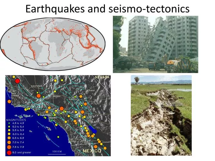
Earthquakes and seismo-tectonics. Elastic rebound model of earthquakes.

E N D
Elastic rebound model of earthquakes An earthquake is a rapid release of stored elastic strain on 1-30 s time-scales. The earthquake happens (nucleates) when the stress on a fault plane exceeds the strength (frictional) of a fault plane in a region. Then, the inertial accelerations can ‘run-away’ to rupture a significant length of the fault plane. Movement of plates (blocks) on either side of fault produce accumulating stress over time. This accumulating stress creates accumulating strain that localizes along the fault plane. The fault brittle strength is exceeded making an earthquake that ruptures and causes the strain energy to be relieved (note straight ‘strain’ lines after rupture).
Locating an earthquake approximately Eq origin time ??? t = x/v Know velocity (v) But don’t know x The arrival-times of the first arriving P-wave is measured. From this arrival-time measurement we now know that station (A) is closest to the earthquake and station (B) the farthest away. WHY ? Thus, to honor the travel-time measurements, we know that the earthquake epicentre is somewhere within the shaded region in (b). To locate an earthquake we must ‘solve’ for the location (x,y,z) and origin time. Note this method is very poor for locating the depth below the surface of the earthquake!
Locating earthquake more exactly using P and S arrival times If we know the P- and S-wave velocity structure AND can measure the P- and S-wave arrival times, then the earthquake origin-time and locations can be estimated. The S-P interval time will tell you the distance of the earthquake. Then, a circle can be drawn around the recording station at that distance. Do that for 3 or more S-P interval times and the earthquakes location can be estimated as the intersection ‘point’ of the circular arcs.
Constrain the depth of an earthquake using pP phase The hypocentre is where the earthquake occurred and is denoted by its latitude, longitude and depth. The epicentre is just the latitude and longitude of the earthquake. For an earthquake that occurs at depth (most earthquakes occur between 10-40 km depth), the depth of the earthquake can be constrained by measuring the arrival time of both the first arrival P-wave and the surface reflection phases called little-p big-P (pP). Note that the time separation between P and pP phases increases with the increasing depth of the earthquake.
Force types: linear, couple, double couple linear-force cc force-couple c force-couple double couple Elastic medium Forces Torques A force has direction and magnitude. A linear force is just one force vector. A torque is a rotational force that requires two force vectors and is define as τ=2F*d where d is the ½ length of moment arm. A double couple is two force couples with opposite signs; this means the net torque is ZERO! All earthquakes are double-couples, otherwise angular momentum would NOT be conserved (a mortal sin!). Not confirmed until 1950’s!
Seismic P and S-wave radiation patterns to applied force impulse (hammer blow) When a force is applied over a finite time, the force-impulse (F*∆t) excites radiation of seismic (elastic) waves. (a) The direction of the hammer impulse makes the rock to the north compress and the rock to the south dilitate which is the P-wave. S-wave radiate to the E and W. (b) Given the direction of the force-impulse (hammer blow), the first motion recorded by station to the north will be compressive, and conversely the first motion recorded to the south will be dilitational. (c) S-wave radiation pattern is a maximum in the E and W directions. As always S-waves are transverse waves.
Earthquake double couple force The force system driving an earthquake is a double couple. WHY ? The fault plane, its displacement, and the auxiliary fault plane. The P-wave radiation pattern. (+) defines compressional (up) first motion and (-) defines dilitational (down) first motion. The double couple force that drives the earthquake defines a compression and tension axis at 45⁰ angle to the fault and auxiliary planes.
First motion of P-wave Important: from the seismic first motion analysis it is IMPOSSIBLE to know which of the two planes is the one that ruptures (the fault plane). One must use other information to resolve the fault plane ambiguity.
Lower hemisphere focal sphere To handle arbitrary fault planes in 3-dimensions, a sphere is place around the earthquake hypocentre. The sphere is oriented with respect to the cardinal directions. Shows the fault and auxiliary fault planes (strike and dip). (b) Because 3-d drawing are a pain, a lower hemisphere projection is used to exactly represent the geometry in (a). The hypocenter is at the middle of the ‘beach-ball’ and the fault and its auxiliary plane are shown. The P-wave first-motion for rays going downwards are shaded gray (compressional) and white (dilatational).
Different fault types: normal, thrust, strike-slip Different fault types make different beach-ball patters of compression and dilitation. Note that the normal and thrust fault planes are the same but the pattern of compression/dilitation is reversed!
Max/min stress axes orientation and fault type σ1 Maximum stress axis σ3 Minimum stress axis σ2 Intermediate stress axis
Finding ‘best’ fault/auxiliary fault plane using measured first-motions and ‘stereonet’ analysis
Double couples again Single couple Single couple Rotation WRONG! Double couple force equivalent The double couple is equivalent to a compressional stress axis (C-C’) and a tensional (dilatational) stress axis (P-P’)! Double couple
Rupture dimensions and displacement A fault is often described by three parameters: a plane with a width (W) and length (L) and the average displacement (D) that occur on the fault plane.
Earthquake (main shock) and after-shocks After a significant size earthquake, residual stress exists that cause small magntitude earthquakes called ‘after-shocks’. These aftershock can be used to map the vertical and lateral extent (i.e., spatial size) of the main-shock.
Measuring ground displacement from GPS to constrain fault plane size The number are in meters (m) of horizontal displacement caused by the quake.
Definition of seismic moment The definition of the moment for a linear force is M = F*d (N-m). The definition of the moment of a force couple is: M = F*2b (N-m). Seismic moment is how seismologist represent the size (energy) of a quake.
Use of Rayleigh and Love (surface) waves to estimate earthquake focal mechanism and moment Using the recorded surface waves to measure earthquake parameters is easy to do and routine. Within seconds after the waves from any earthquake larger than magnitude 5.5 are recorded, an automatic focal mechanism and moment estimate (magnitude) are calculated and sent out as real-time warnings.
A simple definition of seismic magnitude (relative scale) If one can estimate the distance to the quake using the S-P time and the peak Amplitude of the S-wave, a seismic magnitude (not moment) can be calculated.
Regional seismic moment analysis By adding up all the seismic moment measured from seismograms, one can check to see if the earthquakes are accommodating most of the measured displacement (e.g., from GPS). It turns out that this analysis shows that most of the displacement is accommodated by earthquakes. However, rarely a fault does NOT make big earthquake, but instead ‘creeps’ and only makes many small quakes. e.g., the creeping section of the San Andreas fault shown at left.
Rupture length and seismic moment scaling (b) Shows that larger earthquake (bigger moments) have bigger ruptuer lengths. This is called a scaling. It means that big displacements do NOT happen on small fault planes!
Scaling between energy and moment magnitude This shows the relation between moment magnitude and energy. On a log base 10 scale (a), the moment versus energy relation is a straight line. This means that moment magnitude is a logarithmic scale (as defined!).
Guttenberg-Richter scaling relation This straight line relation between the logarithm of the number of earthquakes and their magnitude is called the Guttenberg-Richter relation. This means that are A LOT more small earthquakes than biggers: e.g., there are a 100,000 magnitude 4 quakes for every magnitude 8 quake! A deep physics finding from this ‘power law’ relation is that earthquakes are a manifestation of a ‘self-organized critical system’.
Real-time global seismic network Earthquakes are computer detected and located without about 5 sec after P-waves arrive to guide damage estimates and provide tsunami warnings.
So. California Earthquake ruptureSouth California 3-d earthquake.movseismic earth waves homo.avi