Download

1 / 28
280 likes | 407 Views
MEGN 537 – Probabilistic Biomechanics Ch.1 – Introduction Ch.2 – Mathematics of Probability. Anthony J Petrella, PhD. Ch.1 - Introduction. Uncertainty. Uncertainty present in physical systems Repeated measurement yields variability

E N D
MEGN 537 – Probabilistic BiomechanicsCh.1 – Introduction Ch.2 – Mathematics of Probability Anthony J Petrella, PhD
Uncertainty • Uncertainty present in physical systems • Repeated measurement yields variability • Dimensional tolerances, respiration rate, tissue material properties, joint loading, etc. • What impact does this uncertainty have on performance?
Strength-Based Reliability • Safety factor shows acceptable design • Some percentage of the time, stress may exceed strength
Reliability Definitions • Probability of Failure • POF = 0.001, 0.0001 • Probability of Survival or Reliability • Reliability = 0.999 (three 9s), 0.9999 (four 9s) • POF + POS = 1
Reliability-based Design • Design for Six Sigma • Concept developed by Bill Smith in 1993 • Motorola owns six sigma trademark • Six sigma corresponds to 3.4 failures per 1,000,000 • POF = 0.000,003,4 or Reliability = 0.999,997,6 • Design Excellence or BlackBelt programs • Many companies have implemented their versions • GE and Honeywell boast 100s of millions of dollars saved
Uncertainty • Sources of uncertainty • Inherent / repeated measurement • Statistical uncertainty – limited availability of sampling size means actual distribution unknown • Modeling uncertainty – how good is the model? • Cognitive or qualitative sources – intellectual abstraction of reality, human factors
Course Objectives • Ability to understand and apply probability theory and probabilistic analysis methods • To assess impact of uncertainty in parameters (inputs) on performance (outcomes) • Determine the appropriate distribution to represent a dataset • To apply this knowledge to real biomechanical systems
Definitions • Probability: The likelihood of an event occurring • Event: Represents the outcome of a single experiment (or single simulation) • Experiment: An occurrence that has an uncertain outcome (die toss , coin toss, tensile test) – usually based on a physical model • Simulation: An occurrence that has an uncertain outcome – usually based on an analytical or computational model
Example – Coin Toss • OR = add, AND = multiply • If you flip a coin two times, what is the probability of: • seeing “heads” one time? • seeing “heads” two times?
Example – Coin Toss • OR = add, AND = multiply • If you flip a coin two times, what is the probability of : • seeing “heads” one time? option 1: heads (0.5) AND tails (0.5) = 0.25option 2: tails (0.5) AND heads (0.5) = 0.25option 1 OR option 2 = 0.25 + 0.25 = 0.5 • seeing “heads” two times? option 1: heads (0.5) AND heads (0.5) = 0.25
Example – TKR Casting • A knee implant casting process is known to produce a defective part 5% of the timeIf 10 castings were tested, find the probability of: a) no defective parts b) exactly one defective part c) at least one defective part d) no more than one defective part
Number of permutations of r objects from a set of n distinct objects (ordered sequence) Number of combinations in which r objects can be selected from a set of n distinct objects n objects taken r at a time Independent of order Permutations & Combinations
Must consider combinations for each # of defects Example – Answers
Example - Answers • no defective parts b) exactly one defective part P(0 defects) = P(part 1 no defect)*P(part 2 no defect)… = (1-0.05)^10 = 0.598 P(1 defect) = P(part 1 defect)*P(part 2 no defect)… = (0.05)*(0.95)^9 *10 = 0.315
Example - Answers c) at least one defective part d) no more than one defective part P(≥ 1 defect) = P(1defect) + P(2 defects) + P(3 defects)… = 1- P(0 defects) = 1-0.598 = 0.402 P(≤ 1 defect) = P(0 defects) + P(1 defect) = 0.598 + 0.315 = 0.913
Definitions • Sample Space (S): The set of all basic outcomes of an experiment • Mutually Exclusive: Events that preclude occurrence of one another • Collectively Exhaustive: No other events are possible S A B
Probability Relations • Experimental outcomes can be represented by set theory relationships • Union: A1A3, elements belong to A1 or A3 or both • P(A1A3) = P(A1) + P(A3) - P(A1A3) = A1+A3-A2 • Intersection: A1A3, elements belong to A1 and A3 • P(A1A3) = P(A3|A1) * P(A1) = A2 (multiplication rule) • Complement: A’, elements that do not belong to A • P(A’) = 1 – P(A) S
Special Cases • If the events are statistically independent • P(AB) = P(B|A) * P(A) = P(B) * P(A) • If the events are mutually exclusive • P(AB) = 0 • P(AB) = P(A) + P(B) - P(AB) = P(A) + P(B) S A B
Example • For a randomly chosen automobile:Let A={car has 4 cylinders} B={car has 6 cylinders}. Since events are mutually exclusive, if B occurs, then A cannot occur. So P(A|B) = 0 ≠ P(A). • If 2 events are mutually exclusive, they cannot be independent…when A & B are mutually exclusive, the information that A occurred says something about B (it cannot have occurred), so independence is precluded
Rules of Set Theory • Commutative:AB = BA, AB = BA • Associative:(AB)C = A(BC) • Distributive:(AB)C = (AC)(BC) • Complementary:P(A) + P(A’) = 1 • de Morgan’s Rule: • (AB)’ = A’B’ Complement of union = intersection of complements • (A B)’ = A’ B’ Complement of intersection = union of complements
Conditional Probability • The likelihood that event B will occur if event A has already occurred • P(AB) = P(B|A) * P(A) • P(B|A) = P(AB) / P(A) • Requires that P(A) ≠ 0 • Multiplication Rule: • P(AB) = P(A|B) * P(B) = P(B|A) * P(A) S A B
Example • Common knee injuries include: PCL tear (A), MCL sprain (B), meniscus tear (C) • Injury statistics as reported by epidemiology literature: a) What does the Venn Diagram look like?
Example S A B 0.02 0.07 0.03 0.05 0.04 0.08 0.20 0.51 C
Example b) What is the probability that a patient with an MCL sprain (B) will later sustain a PCL tear (A)? S A B 0.02 0.07 0.03 0.05 0.04 0.08 0.20 P(A|B) = P(A B) = 0.08 = 0.348 P(B) 0.23 0.51 C
Example c) If a patient has sustained either an MCL sprain (B) or a meniscus tear (C) or both, what is the probability of a later PCL tear (A)? S A B 0.02 0.07 0.03 0.05 0.04 0.08 0.20 P(A| BC) = P(A (BC) = 0.03+0.04+0.05 = 0.26 P(BC) 0.47 0.51 C
Example d) If a patient has sustained at least one knee injury in the past, what is the probability he will later tear his PCL? P(A|at least one) = P(A | ABC) = P(A (ABC) P(ABC) P(A (ABC) = P(A) = 0.14 = 0.28 P(ABC) P(ABC) 0.49