Download
1 / 31
310 likes | 448 Views
Fast optimal instruction scheduling for single-issue processors with arbitrary latencies Peter van Beek, University of Waterloo Kent Wilken, University of California, Davis CP 2001 · Paphos, Cyprus November 2001. Local instruction scheduling. Schedule basic-block

E N D
Fast optimal instruction scheduling for single-issue processors with arbitrary latenciesPeter van Beek, University of WaterlooKent Wilken, University of California, DavisCP 2001 · Paphos, CyprusNovember 2001
Local instruction scheduling • Schedule basic-block • straight-line sequence of code with single entry, single exit • Single-issue pipelined processors • single instruction can begin execution each clock cycle • delay or latencybefore result is available • Classic problem • lots of attention in literature • Remains important • single-issue RISC processors used in embedded systems 2
dependency DAG A B 3 3 D C 1 3 E Example: evaluate (a + b) + c instructions A r1 a B r2 b C r3 c D r1 r1 + r2 E r1 r1 + r3 3
dependency DAG A B 3 3 D C 1 3 E Example: evaluate (a + b) + c non-optimal schedule A r1 a B r2 b nop nop D r1 r1 + r2 C r3 c nop nop E r1 r1 + r3 4
dependency DAG A B 3 3 D C 1 3 E Example: evaluate (a + b) + c optimal schedule A r1 a B r2 b C r3 c nop D r1 r1 + r2 E r1 r1 + r3 5
Local instruction scheduling problem • Given a labeled dependency DAG G = (N, E) for a basic block, find a schedule S that specifies a start time S( i ) for each instruction such that • S( i ) S( j ), i, j N, i j, • and • S( j ) S( i ) + latency( i, j ), ( i, j ) E, • and • max{ S( i ) | i N } is minimized. 6
Previous work • NP-Complete if arbitrary latencies (Hennessy & Gross, 1983; Palem & Simons, 1993) • Polynomial special cases (Bernstein & Gertner, 1989; Palem & Simons, 1993; Wu et al., 2000) • Optimal algorithms • dynamic programming (e.g., Kessler, 1998) • integer linear programming (e.g., Wilken et al., 2000) • constraint programming (e.g., Ertl & Krall, 1991) 7
dependency DAG A B 3 3 D C 1 3 E Minimal constraint model variables A, B, C, D, E domains {1, …, m} constraints D A + 3 D B + 3 E C + 3 E D + 1 all-diff(A, B, C, D, E) 8
[1, 2] [1, 2] [3, 3] [4, 5] [6, 6] Bounds consistency For each constraint C and for each variable x in C, min has a support in C and max has a support in C variable A B C D E domain [1, 6] [1, 6] [1, 6] [1, 6] [1, 6] constraints [1, 3] D A + 3 D B + 3 E C + 3 E D + 1 all-diff(A, B, C, D, E) [4, 6] 9
Three improvements to minimal model • 1. Initial distance constraints • defined over nodes which define regions • 2. Improved distance constraints for small regions • 3. Predecessor and successor constraints • defined over nodes with multiple predecessors or multiple successors 10
Three improvements to minimal model • 1. Initial distance constraints • defined over nodes which define regions • 2. Improved distance constraints for small regions • 3. Predecessor and successor constraints • defined over nodes with multiple predecessors or multiple successors 11
Distance constraints: Regions A pair of nodes i, j define a region in a DAG G if: (i) there is more than one path from i to j, and (ii) not all paths from i to j go through some node k distinct from i and j. 12
A 1 1 C B 3 3 D E 1 1 1 F G 3 3 H Distance constraints: Initial estimate 13
A 1 1 A F j+1 j C B j+2 j+3 j+4 j+5 3 3 5 D E 1 1 1 F G 3 3 H Distance constraints: Initial estimate 14
A 1 1 E H j+1 j C B j+2 j+3 j+4 j+5 3 3 D E 1 1 1 F 5 G 3 3 H Distance constraints: Initial estimate 15
A 1 1 A H j+6 j+1 j C B j+2 j+3 j+4 j+5 3 3 D E j+7 j+8 j+9 1 1 1 F G 9 3 3 H Distance constraints: Initial estimate 16
Three improvements to minimal model • 1. Initial distance constraints • defined over nodes which define regions • 2. Improved distance constraints for small regions • 3. Predecessor and successor constraints • defined over nodes with multiple predecessors or multiple successors 17
[1,1] A 1 1 [2,3] [2,3] C B 3 3 [5,6] [5,6] D E 1 1 1 [6,7] [6,7] F G 3 3 [10,10] H Improved distance constraints for small regions • Given H A + 9 • Extract region from DAG • Post constraints • Test consistency of A 1 H 10 propagate latency propagate all-diff 18
[1,1] • Given H A + 9 A 1 1 • Extract region from DAG • Post constraints [2,3] [2,3] C B • Test consistency of A 1 H 10 3 3 [5,6] [5,6] D E 1 1 1 propagate latency [6,7] [6,7] F G propagate all-diff 3 3 [10,10] H Improved distance constraints for small regions inconsistent • Repeat with H A + 10 19
Three improvements to minimal model • 1. Initial distance constraints • defined over nodes which define regions • 2. Improved distance constraints for small regions • 3. Predecessor and successor constraints • defined over nodes with multiple predecessors or multiple successors 20
A 7 1 G B F 1 [5,8] 1 1 D H [6,9] [5,9] [5,9] C 3 3 3 [8,12] [9,12] E 2 2 11 Predecessor constraints [4, ] [ ,14] 21
A [4, ] 7 1 6 5 G B F 1 [5,8] 1 7 8 9 1 H [6,9] [5,9] [5,9] D C 3 3 3 [8,12] [9,12] E 2 2 [ ,14] 11 Predecessor constraints [9,12] 22
A [4, ] 7 1 9 G B 1 [5,8] 1 10 11 12 1 D [6,9] [5,9] [5,9] C 3 3 3 [8,12] [9,12] F [9,12] E 2 2 [ ,14] 11 H Predecessor constraints [12,14] 23
[4, ] 7 A 1 6 1 [5,8] B 1 7 8 9 1 [6,9] [5,9] [5,9] C D E 3 3 3 [8,12] [9,12] F G [9,12] 2 2 [12,14] [ ,14] 11 H Successor constraints [4,6] 24
Solving instances of the model • Use constraints to establish: • lower bound on length m of optimal schedule • lower and upper bounds of variables • Backtracking search • maintains bounds consistency • Puget’s (1998) all-diff propagator and optimizations • Leconte’s (1996) optimizations • branches on lower(x), lower(x)+1, … • If no solution found, increment m and repeat search 25
Experimental results • Embedded in Gnu Compiler Collection (GCC) • Compared with: • GCC’s critical path list scheduling • ILP scheduler (Wilken et al., 2000) • SPEC95 floating point benchmarks • compiled using highest level of optimization (-O3) • Target processor: • single-issue • latency of 3 for loads, 2 for floating point, 1 for integer ops 26
Experimental results: SPEC95 floating point benchmarks Total basic blocks (BB) BB passed to CSP scheduler BB solved optimally by CSP scheduler BB with improved schedule Static cycles improved Total benchmark cycles CSP scheduling time (sec.) Baseline compile time (sec.) 7,402 517 517 29 66 107,245 4.5 708 27
Quantifying contributions ofthree model improvements Problems solved (/15) 29
Conclusions • CP approach to local instruction scheduling • single-issue processors • arbitrary latencies • Optimal and fast on very large, real problems • experimental evaluation on SPEC95 benchmarks • 20-fold improvement over previous best approach • Key was an improved constraint model 30
Good ideas not included • Cycle cutsets (e.g., Dechter, 1990) • most larger problems had small cutsets (2 to 20 nodes) that split problem into equal-sized independent subproblems • Singleton consistency (e.g., Prosser et al., 2000) • often reduced domains dramatically prior to search • Symmetry breaking constraints • many symmetric (non) schedules 31