Download
1 / 14
140 likes | 222 Views
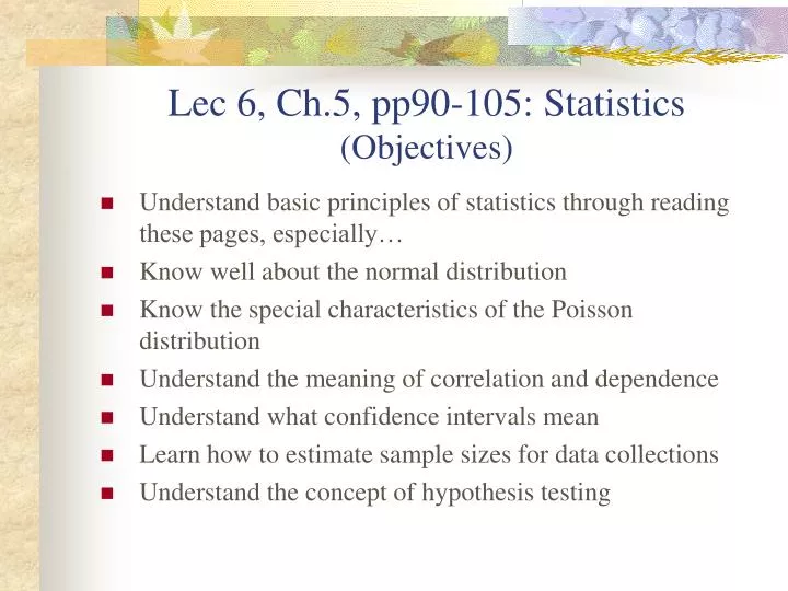
Lec 6, Ch.5, pp90-105: Statistics (Objectives). Understand basic principles of statistics through reading these pages, especially… Know well about the normal distribution Know the special characteristics of the Poisson distribution Understand the meaning of correlation and dependence

E N D
Lec 6, Ch.5, pp90-105: Statistics (Objectives) • Understand basic principles of statistics through reading these pages, especially… • Know well about the normal distribution • Know the special characteristics of the Poisson distribution • Understand the meaning of correlation and dependence • Understand what confidence intervals mean • Learn how to estimate sample sizes for data collections • Understand the concept of hypothesis testing
What we cover in class today… Anything not covered in class, you learn them from reading pp.95-105. • The normal distribution – how to read the standard normal distribution table • Central limit theory (CLT) • The Poisson distribution – why it is relevant to traffic engineering • Correlation and dependence • Confidence bounds and their implications • Estimating sample sizes • The concept of hypothesis testing
The normal distribution Mean = 55 mph What’s the probability the next value will be less than 65 mph? z = (x - µ)/ = (65 – 55)/7 = 1.43 From the sample normal distribution to the standard normal distribution.
Use of the standard normal distribution table, Tab 5-1 Z = 1.43 Most popular one is 95% within µ ± 1.96
Central limit theorem (CLT) Definition: The population may have any unknown distribution with a mean µ and a finite variance of 2. Take samples of sizen from the population. As the size of n increases, the distribution of sample means will approach a normal distribution with mean µ and a variance of 2/n. F(x) approaches x µ µ X distribution X ~ any (µ, 2) distribution
The Poisson distribution (“counting distribution” or “Random arrival”) With mean µ = m and variance 2 = m. If the above characteristic is not met, the Poisson does not apply. • The binomial distribution tends to approach the Poisson distribution with parameter m = np. (See Table 4-3) • When time headways are exponentially distributed with mean = 1/, the number of arrivals in an interval T is Poisson distributed with mean = m = T.
Correlation and dependence y = f(x) Linear regression: y = a + bx Non-linear regression: y = axb(example) Dependent variable y Correlation coefficient r (1, perfect fit) Coefficient of determination r2 (Tells you how much of variability can be “explained” by the independent variables.) Independent variable x
X X Confidence bounds and interval Point estimates: A point estimate is a single-values estimate of a population parameter made from a sample. Interval estimates: An interval estimate is a probability statement that a population parameter is between two computed values (bounds). µ True population mean - - Point estimate of X from a sample Two-sided interval estimate X – tas/sqrt(n) X + tas/sqrt(n)
Confidence interval (cont) When n gets larger (n>=30), t can become z. The probability of any random variable being within 1.96 standard deviations of the mean is 0.95, written as: P[(µ - 1.96) y (µ + 1.96)] = 0.95 Obviously we do not know µ and . Hence we restate this in terms of the distribution of sample means: P[( x - 1.96E) y ( x + 1.96E)] = 0.95 Where, E = s/SQRT(n) (Review 1, 2, 3, and 4 in page 100.)
Estimating sample sizes For cases in which the distribution of means can be considered normal, the confidence range for 95% confidence is: If this value is called the tolerance (or “precision”), and given the symbol e, then the following equation can be solved for n, the desired sample size: and By replacing 1.96 with z and 3.84 with z2, we can use this for any level of confidence. (Review 1 and 2 on page 101.)
The concept of hypothesis testing Two distinct choices: Null hypothesis, H0 Alternative hypothesis: H1 E.g. Inspect 100,000 vehicles, of which 10,000 vehicles are “unsafe.” This is the fact given to us. H0: The vehicle being tested is “safe.” H1: The vehicle being tested is “unsafe.” In this inspection, 15% of the unsafe vehicles are determined to be safe Type II error (bad error) and 5% of the safe vehicles are determined to be unsafe Type I error (economically bad but safety-wise it is better than Type II error.)
Types of errors We want to minimize especially Type II error. Steps of the Hypothesis Testing Decision Reality Reject H0 Accept H0 • State the hypothesis • Select the significance level • Compute sample statistics and estimate parameters • Compute the test statistic • Determine the acceptance and critical region of the test statistics • Reject or do not reject H0 H0 is true Type I error Correct Correct Type II error H1 is true Fail to reject a false null hypothesis Reject a correct null hypothesis P(type I error) = (level of significance) P(type II error ) =
Dependence between , , and sample size n There is a distinct relationship between the two probability values and and the sample size n for any hypothesis. The value of any one is found by using the test statistic and set values of the other two. • Given and n, determine . Usually the and n values are the most crucial, so they are established and the value is not controlled. • Given and , determine n. Set up the test statistic for and with H0 value and an H1 value of the parameter and two different n values. The t (or z) statistics is: t or z (Use an example from a stat book)
One-sided and two-sided tests • The significance of the hypothesis test is indicated by , the type I error probability. = 0.05 is most common: there is a 5% level of significance, which means that on the average a type I error (reject a true H0) will occur 5 in 100 times that H0 and H1 are tested. In addition, there is a 95% confidence level that the result is correct. 0.025 each • If H1 involves a not-equal relation, no direction is given, so the significance area is equally divided between the two tails of the testing distribution. Two-sided • If it is known that the parameter can go in only one direction, a one-sided test is performed, so the significance area is in one tail of the distribution. 0.05 One-sided upper