Download
1 / 209
2.69k likes | 3.73k Views
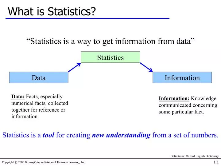
What is Statistics?. “Statistics is a way to get information from data”. Statistics. Data. Information. Data: Facts, especially numerical facts, collected together for reference or information. Information: Knowledge communicated concerning some particular fact.

E N D
What is Statistics? • “Statistics is a way to get information from data” Statistics Data Information Data:Facts, especially numerical facts, collected together for reference or information. Information:Knowledge communicated concerning some particular fact. Statistics is a tool for creating new understanding from a set of numbers. Definitions: Oxford English Dictionary
Key Statistical Concepts… • Population • — a population is the group of all items of interest to a statistics practitioner. • — frequently very large; sometimes infinite. • E.g. All 5 million Florida voters, per Example 12.5 • Sample • — A sample is a set of data drawn from the population. • — Potentially very large, but less than the population. • E.g. a sample of 765 voters exit polled on election day.
Key Statistical Concepts… • Parameter • — A descriptive measure of a population. • Statistic • — A descriptive measure of a sample.
Key Statistical Concepts… Population • Populations have Parameters, • Samples have Statistics. Sample Subset Statistic Parameter
Descriptive Statistics… • …are methods of organizing, summarizing, and presenting data in a convenient and informative way. These methods include: • Graphical Techniques (Chapter 2), and • Numerical Techniques (Chapter 4). • The actual method used depends on what information we would like to extract. Are we interested in… • • measure(s) of central location? and/or • • measure(s) of variability (dispersion)? • Descriptive Statistics helps to answer these questions…
Statistical Inference… • Statistical inference is the process of making an estimate, prediction, or decision about a population based on a sample. Population Sample Inference Statistic Parameter What can we infer about a Population’s Parameters based on a Sample’s Statistics?
Definitions… • A variable is some characteristic of a population or sample. • E.g. student grades. • Typically denoted with a capital letter: X, Y, Z… • The valuesof the variable are the range of possible values for a variable. • E.g. student marks (0..100) • Data are the observed values of a variable. • E.g. student marks: {67, 74, 71, 83, 93, 55, 48}
Interval Data… • Intervaldata • • Real numbers, i.e. heights, weights, prices, etc. • • Also referred to as quantitative or numerical. • Arithmetic operations can be performed on Interval Data, thus its meaningful to talk about 2*Height, or Price + $1, and so on.
Nominal Data… • Nominal Data • • Thevalues of nominal data are categories. • E.g. responses to questions about marital status, coded as: • Single = 1, Married = 2, Divorced = 3, Widowed = 4 • Because the numbers are arbitrary arithmetic operations don’t make any sense (e.g. does Widowed ÷ 2 = Married?!) • Nominal data are also called qualitative or categorical.
Ordinal Data… • OrdinalData appear to be categorical in nature, but their values have an order; a ranking to them: • E.g. College course rating system: • poor = 1, fair = 2, good = 3, very good = 4, excellent = 5 • While its still not meaningful to do arithmetic on this data (e.g. does 2*fair = very good?!), we can say things like: • excellent > poor or fair < very good • That is, order is maintained no matter what numeric values are assigned to each category.
Graphical & Tabular Techniques for Nominal Data… • The only allowable calculation on nominal data is to count the frequency of each value of the variable. • We can summarize the data in a table that presents the categories and their counts called a frequency distribution. • A relative frequency distribution lists the categories and the proportion with which each occurs. • Refer to Example 2.1
Nominal Data (Frequency) Bar Charts are often used to display frequencies…
Nominal Data It all the same information, (based on the same data). Just different presentation.
Graphical Techniques for Interval Data • There are several graphical methods that are used when the data are interval (i.e. numeric, non-categorical). • The most important of these graphical methods is the histogram. • The histogram is not only a powerful graphical technique used to summarize interval data, but it is also used to help explain probabilities.
Building a Histogram… • Collect the Data • Create a frequency distribution for the data. • Draw the Histogram.
Ogive… • Is a graph of a cumulativefrequency distribution. • We create an ogive in three steps… • 1) Calculate relative frequencies. • 2) Calculate cumulative relative frequencies by adding the current class’ relative frequency to the previous class’ cumulative relative frequency. • (For the first class, its cumulative relative frequency is just its relative frequency)
Cumulative Relative Frequencies… first class… next class: .355+.185=.540 : : last class: .930+.070=1.00
Ogive… The ogive can be used to answer questions like: What telephone bill value is at the 50th percentile? “around $35” (Refer also to Fig. 2.13 in your textbook)
Scatter Diagram… • Example 2.9 A real estate agent wanted to know to what extent the selling price of a home is related to its size… • Collect the data • Determine the independent variable (X – house size) and the dependent variable (Y – selling price) • Use Excel to create a “scatter diagram”…
Scatter Diagram… • It appears that in fact there is a relationship, that is, the greater the house size the greater the selling price…
Patterns of Scatter Diagrams… • Linearity and Direction are two concepts we are interested in Positive Linear Relationship Negative Linear Relationship Weak or Non-Linear Relationship
Time Series Data… • Observations measured at the same point in time are called cross-sectional data. • Observations measured at successive points in time are called time-series data. • Time-series data graphed on a line chart, which plots the value of the variable on the vertical axis against the time periods on the horizontal axis.
Numerical Descriptive Techniques… • Measures of Central Location • Mean, Median, Mode • Measures of Variability • Range, Standard Deviation, Variance, Coefficient of Variation • Measures of Relative Standing • Percentiles, Quartiles • Measures of Linear Relationship • Covariance, Correlation, Least Squares Line
Measures of Central Location… • The arithmetic mean, a.k.a. average, shortened to mean, is the most popular & useful measure of central location. • It is computed by simply adding up all the observations and dividing by the total number of observations: Sum of the observations Number of observations Mean =
Arithmetic Mean… Sample Mean Population Mean
The Arithmetic Mean… • …is appropriate for describing measurement data, e.g. heights of people, marks of student papers, etc. • …is seriously affected by extreme values called “outliers”. E.g. as soon as a billionaire moves into a neighborhood, the average household income increases beyond what it was previously!
Measures of Variability… • Measures of central location fail to tell the whole story about the distribution; that is, how much are the observations spread out around the mean value? For example, two sets of class grades are shown. The mean (=50) is the same in each case… But, the red class has greater variability than the blue class.
Range… • The range is the simplest measure of variability, calculated as: • Range = Largest observation – Smallest observation • E.g. • Data: {4, 4, 4, 4, 50} Range = 46 • Data: {4, 8, 15, 24, 39, 50} Range = 46 • The range is the same in both cases, • but the data sets have very different distributions…
Variance… • The variance of a population is: • The variance of a sample is: population mean population size sample mean Note! the denominator is sample size (n) minus one !
Application… • Example 4.7. The following sample consists of the number of jobs six randomly selected students applied for: 17, 15, 23, 7, 9, 13. • Finds its mean and variance. • What are we looking to calculate? • The following sample consists of the number of jobs six randomly selected students applied for: 17, 15, 23, 7, 9, 13. • Finds its mean and variance. …as opposed to or 2
Sample Mean & Variance… Sample Mean Sample Variance Sample Variance (shortcut method)
Standard Deviation… • The standard deviation is simply the square root of the variance, thus: • Population standard deviation: • Sample standard deviation:
Standard Deviation… • Consider Example 4.8 where a golf club manufacturer has designed a new club and wants to determine if it is hit more consistently (i.e. with less variability) than with an old club. • Using Tools > Data Analysis [may need to “add in”… > Descriptive Statistics in Excel, we produce the following tables for interpretation… You get more consistent distance with the new club.
The Empirical Rule… If the histogram is bell shaped • Approximately 68% of all observations fall • within one standard deviation of the mean. • Approximately 95% of all observations fall • within two standard deviations of the mean. • Approximately 99.7% of all observations fall • within three standard deviations of the mean.
Chebysheff’s Theorem…Not often used because interval is very wide. • A more general interpretation of the standard deviation is derived from Chebysheff’s Theorem, which applies to all shapes of histograms (not just bell shaped). • The proportion of observations in any sample that lie • within k standard deviations of the mean is at least: For k=2 (say), the theorem states that at least 3/4 of all observations lie within 2 standard deviations of the mean. This is a “lower bound” compared to Empirical Rule’s approximation (95%).
Box Plots… • These box plots are based on data in Xm04-15. • Wendy’s service time is shortest and least variable. • Hardee’s has the greatest variability, while Jack-in-the-Box has the longest service times.
Methods of Collecting Data… • There are many methods used to collect or obtain data for statistical analysis. Three of the most popular methods are: • • Direct Observation • • Experiments, and • • Surveys.
Sampling… • Recall that statistical inference permits us to draw conclusions about a population based on a sample. • Sampling (i.e. selecting a sub-set of a whole population) is often done for reasons of cost (it’s less expensive to sample 1,000 television viewers than 100 million TV viewers) and practicality (e.g. performing a crash test on every automobile produced is impractical). • In any case, the sampled population and the target population should be similar to one another.
Sampling Plans… • A sampling plan is just a method or procedure for specifying how a sample will be taken from a population. • We will focus our attention on these three methods: • Simple Random Sampling, • Stratified Random Sampling, and • Cluster Sampling.
Simple Random Sampling… • A simple random sample is a sample selected in such a way that every possible sample of the same size is equally likely to be chosen. • Drawing three names from a hat containing all the names of the students in the class is an example of a simple random sample: any group of three names is as equally likely as picking any other group of three names.
Stratified Random Sampling… • After the population has been stratified, we can use simple random sampling to generate the complete sample: If we only have sufficient resources to sample 400 people total, we would draw 100 of them from the low income group… …if we are sampling 1000 people, we’d draw 50 of them from the high income group.
Cluster Sampling… • A cluster sample is a simple random sample of groups or clusters of elements (vs. a simple random sample of individual objects). • This method is useful when it is difficult or costly to develop a complete list of the population members or when the population elements are widely dispersed geographically. • Cluster sampling may increase sampling error due to similarities among cluster members.
Sampling Error… • Sampling error refers to differences between the sample and the population that exist only because of the observations that happened to be selected for the sample. • Another way to look at this is: the differences in results for different samples (of the same size) is due to sampling error: • E.g. Two samples of size 10 of 1,000 households. If we happened to get the highest income level data points in our first sample and all the lowest income levels in the second, this delta is due to sampling error.
Nonsampling Error… • Nonsampling errors are more serious and are due to mistakes made in the acquisition of data or due to the sample observations being selected improperly. Three types of nonsampling errors: • Errors in data acquisition, • Nonresponse errors, and • Selection bias. • Note: increasing the sample size will not reduce this type of error.
Approaches to Assigning Probabilities… • There are three ways to assign a probability, P(Oi), to an outcome, Oi, namely: • Classical approach: make certain assumptions (such as equally likely, independence) about situation. • Relative frequency: assigning probabilities based on experimentation or historical data. • Subjective approach: Assigning probabilities based on the assignor’s judgment.
Interpreting Probability… • One way to interpret probability is this: • If a random experiment is repeated an infinite number of times, the relative frequency for any given outcome is the probability of this outcome. • For example, the probability of heads in flip of a balanced coin is .5, determined using the classical approach. The probability is interpreted as being the long-term relative frequency of heads if the coin is flipped an infinite number of times.