Download
1 / 28
280 likes | 444 Views
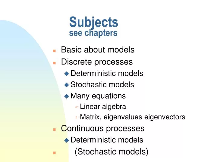
Subjects see chapters. Basic about models Discrete processes Deterministic models Stochastic models Many equations Linear algebra Matrix , eigenvalues eigenvectors Continuous processes Deterministic models ( Stochastic models). Stages, States and Classes.

E N D
Subjectsseechapters • Basic about models • Discrete processes • Deterministic models • Stochastic models • Manyequations • Linear algebra • Matrix, eigenvalues eigenvectors • Continuous processes • Deterministic models • (Stochastic models)
Stages, States and Classes • Can we always treat a population as a single entity? • Do we need to divide it into different stages or classes? • Age-classes • Size-classes • Subdivided in space • Morphological classes • The subpopulations (stages-classes) differ from each other in aspects important for the purpose and dynamics of the modell. For example in fecundity, survival, dispersal, or risk of predation, or environmental variation, or….. Specific example. Young individuals give birth to fewer than mean aged individuals
Stages, States andClasses • We can use linear algebra, matrix calculations to: • Determine equlibriums (eigenvectors) • Time to equilibrium. (eigenvalues) • Run simulations (matrix multiplication) • Calculate velocity constants (eigenvalues)
Distribution of thepopulation • A population can be treated as one unity if only number of individuals define its property, for example if 50 individuals give birth to twice as many as 25 do. • If the population has a constant distribution of individuals in its relevant classes/stages, it can be treated as one unity. • For example if it’s always 30% newborns, 20% young, 20% newly reproductive, 20% highly reproductive and 10% postreproductive.
Distribution of thepopulation • n If a population of 50 consist of 10 adults/reproductively mature/ the population will reproduce less then if it consists of 20 adults. If the population varies in proportion of adults it will reproduce differently per capita over time. • If the distribution (proportion in stages/classes) of the population varies over time the population either have to include stages/subpopulation or one have to show that it is reasonable to approximate with a simpler non-stage model.
Distribution of thepopulation The dichotomy Stable proportions of classes/ subpopulations Variation in proportion of individuals in stages/ subpopulations Stable per capita growth rates and dispersal rates etc Variation in per capita growth rates and dispersal rates etc Structured model Non-structured model
Ageclassesmethod: structured population Three ageclasses, n1, n2 och n3. • Next timestep is calculated as n1(t+1)= b1 n1(t)+ b2 n2(t)+ b3n3(t) n2(t+1)= s12 n1(t) n3(t+1)= s23 n2(t) Note, one time step correspondence to size/span of an ageclass. b2 b3 b1 1 2 3 s12 s23 bi = how many newborns from ageclassi during one timestep (span of an ageclass) sij = probability for an individual in age-class ito survive into the next age-class, j
Ageclassesmethod: structured population Three ageclasses, n1, n2 och n3. • Next timestep is calculated as n1(t+1)= b1 n1(t)+ b2 n2(t)+ b3n3(t) n2(t+1)= s12 n1(t) n3(t+1)= s23 n2(t) this is a linear system of equations, one can use linear algebra. Matrix multiplication.
Ageclasses • Next timestep is calculated asn1(t+1)= b1 n1(t)+ b2 n2(t)+ b3n3(t)n2(t+1)= s12 n1(t)n3(t+1)= s23 n2(t)
Ageclasses • Next timestep is calculated asn1(t+1)= b1 n1(t)+ b2 n2(t)+ b3n3(t)n2(t+1)= s12 n1(t)n3(t+1)= s23 n2(t)
Ageclasses, an example • Ageclass 1 do not reproduce • Ageclass 2 give birth to 2 • Ageclass 3 give birth to 8 40% of individuals in ageclass1 survives to ageclass2 80% of individuals in ageclass2 survives to ageclass3 100% of the individuals in agecass3 dies. Start population conisist of 10 young, 8 subadultsand 6 adults..
Ageclasses, matrix multiplication – run a simulation One can calculate this for ever after a while a constant distribution will evolve The right hand side distributions will be the same for all following timesteps Note that the number of individuals may change (density) but the distribution over classes becomes stable densities proportions
Ageclasses, eigenvalues andeigenvectors If the distribution becomes stable then the per capita growth rate also stabilize and becomes a constant value If the per capita growth rate becomes stable/constant over time, one can use that instead of the matrix
Ageclasses, eigenvalues andeigenvectors The other two eigenvalues are complex values and generates the oscillations that occurs prior the stabilisation.
From the beginning again:Solution space and eigenvectors. Assume nay population distribution (not an eigenvector) The lefthand side, vector (59 26 3), exist in a solution space spanned by the three eigenvectors. This means that you can reach the point (59 26 3) in the 3D space by moving along the directions of the three vectors Mathematically this is expressed by:
Solution to n(t)=Atn(0) We know that matris*eigenvector equals eigenvalue*eigenvector Av1=λ1v1. And that: Combine these two and x(t)=Atn(0) can be written as Whathappends at large t (long time???
Stage models b2 b3 • A stage model have classes of different time span, not equals the time step. Hence some of the individuals may stay in the original stage after a timestep. A proportion gimay stay. • Note one have to consider survíval, during one time step, in both p and g parameters. g1 1 2 3 p23 p12 g3 g2
Simple Markov chains More general model • Handles probabilities for an organism to change state, for example running to sleeping or standing or.., healthy to sick to recovered to.. • Can also deal with dispersal. A specific place/habitat is then a state • All numbers are then between 0 and 1 since probability to change from one state to another. • Closed systems, hence no losses or addition.
Simple Markov chains 0.9 • Handles probabilities for an organism to ‘move’ between different states • All numbers along the arrows have to be between 0 and 1 • All numbers out from a state have to sum up to 1. (otherwise a loss or addition) 0.5 0.3 1 3 0.2 0.2 0.1 0.5 2 0.3
Simple Markov chains =1 =1 =1 • A row is the input to a state. • A column is the output of the state. • The row can sum to [0,>1] • The columns always sum to 1 0.9 0.5 0.3 1 3 0.2 0.2 0.1 0.5 2 0.3
Simple Markov chains,absorbing states • A state is absorbing if the probability is 1 to stay in the state. • With time the probability, where the individuals are will move, to this absorbing state. 0.5 0.3 1 3 0.2 0.2 1 0.5 2 0.3
Simple Markov chains,equilibriums • What happends over time? • x(t)=Atx(0)? • Is there any equilibrium, x’=Ax’? • If At after a time t only consist of positive elements (>0), the a equlibriumexists. This equilibrium is the eigenvector with eigenvalue1 of matrix A. • This equilibrium is also a column in At, for large t. At is then the steady state matrix • This equilibrium is a kind of ultimate probability between the states. For example that that there is a 60% probability that an individual is in state 1,….. 0.5 0.3 1 3 0.2 0.2 1 0.5 2 0.3
Simple Markov chains,eigenvalues eigenvectors • An equilibrium exists if all states are connected (direct or indirect). No state is completed isolated. No groups of stesae isolated from the other. • Calculate eigenvectors and eigenvaluesby matlab code, [x,y]=eig(A) • Several equilibriums may exists if there are several absorbing states 0.5 0.3 1 3 0.2 0.2 1 0.5 2 0.3
Absorbing state,equilibrium • It is possible to calculate the probability that a system reaches the different equilibriums • In the example the question is what the probability is to end up in state 2 or three? • More on page 126 and 127, yet this you can read briefly. 0.5 0.3 1 3 0.2 1 2 1
Ageclass/stages Population growth – eigenvalue. Population distribution eigenvector The state of individuals and populations-Markov chains Probability for the state of the individual Equlibrium-eigenvector Summarizingclasses/stages/state-matrices