Download
1 / 25
250 likes | 349 Views
Learn about joint probability density functions for several random variables, conditional PDFs, correlation, covariance, transformations, error propagation, and convolution. Explore examples and applications in data analysis.

E N D
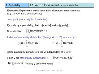
2. Probability 2.3 Joint p.d.f.´s of several random variables Examples: Experiment yields several simultaneous measurements(e.g. temperature and pressure) Joint p.d.f. (here only for 2 variables): f(x,y) dx dy = probability, that x[x,x+dx] and y[y,y+dy] Normalization: Individual probability distribution (“marginal p.d.f.”) for x and y: yields probability density for x (or y) independent of y (or x) x and y are statistically independent if for any y (and vice versa) K. Desch – Statistical methods of data analysis SS10
2. Probability 2.3 Joint p.d.f.´s of several random variables conditional p.d.f.´s: h(y|x)dxdy is the probability for event to lie in the interval [y,y+dy] when the event is known to lie in the interval [x,x+dx]. K. Desch – Statistical methods of data analysis SS10
2. Probability 2.3 Joint p.d.f.´s of several random variables Example: measurement of the length of a bar and its temperature • x = deviation from 800 mm • y = temperature in 0C • 2-dimentional histogram • (“scatter-plot”) • Marginal distribution of y • (“y-projection”) • Marginal distribution of x • (“x-projection”) • 2 conditional distributions of x (s. edges in (a)) • Width in d) smaller than in c) • x and y are “correlated” K. Desch – Statistical methods of data analysis SS10
2. Probability 2.3 Joint p.d.f.´s of several random variables Expectation value (analog to 1-dim. case) Variance (analog to 1-dim. case) important when more than one variable: measure for the correlation of the variables: Covariance for 2 variables x, y with joint p.d.f. f(x,y): if x, y are stat. independent (f(x,y) = fx(x)fy(y)) then cov[x,y] = 0 (but not vice versa!!) K. Desch – Statistical methods of data analysis SS10
2. Probability 2.3 Joint p.d.f.´s of several random variables Positive correlation: positive (negative) deviation of xfrom its x increases the probability, that y has a positive (negative) deiation of its y For the sum of random numbers x+y holds: V[x+y] = V[x] + V[y] + 2 cov[x,y] (proof: linearity of E[]) For n random variables xi i=1,n: is the covariance matrix (symmetric matrix) diagonal elements: For uncorrelated variables: covariance matrix is diagonal For all elements: Normalized quantity: is the correlation coefficient K. Desch – Statistical methods of data analysis SS10
2. Probability 2.3 Joint p.d.f.´s of several random variables examples for correlation coefficients (Axis units play no role !) K. Desch – Statistical methods of data analysis SS10
2. Probability 2.3 Joint p.d.f.´s of several random variables one more example: [Barlow] K. Desch – Statistical methods of data analysis SS10
2. Probability 2.3 Joint p.d.f.´s of several random variables another example: K. Desch – Statistical methods of data analysis SS10
2. Probability 2.4 Transformation of variables Measured quantity: x (distributed according to pdf f(x)) Derived quanitity: y = a(x) What is the p.d.f. of y, g(y) ? Define g(y) by requiring the same probability for y [y,y+dy] a(x) x [x,x+dx] =: dS K. Desch – Statistical methods of data analysis SS10
2. Probability 2.4 Transformation of variables More tedious when x y not a 11 relation, e.g. y two branches x>0 and x<0 for g(y) sum up the probabilities for x>0 and x<0 [y,y+dy] K. Desch – Statistical methods of data analysis SS10
2. Probability 2.Transformation of variables Functions of more variables : transformation through the Jacobian matrix: K. Desch – Statistical methods of data analysis SS10
2. Probability 2.4 Transformation of variables Example: Gaussian momentum distribution Momentum in x and y: polar coordinates x = r cos φ y = r sin φ r2 := x2 + y2 det J = r→ g (r,φ) = f ( x (r,φ), y (r,φ) ) • det J = In 3-dimenions → Maxwell distribution K. Desch – Statistical methods of data analysis SS10
2. Probability 2.5 Error propagation Often, one is not interested in complete transformation of p.d.f. but only in the transformation of its variance (=squared error) measured error of x derived error of y When σx is small relative to curvature of y(x) : → linear approach What about the variance? K. Desch – Statistical methods of data analysis SS10
2. Probability 2.5 Error propagation Variance : → K. Desch – Statistical methods of data analysis SS10
2. Probability 2.5 Error propagation For more variables yi: → general formula for error propagation (in linear approximation) Special cases: a) uncorrelated xj : and even if xi are uncorrelated, the yi are in general correlated K. Desch – Statistical methods of data analysis SS10
2. Probability 2.5 Error propagation b) Sum y =x1+x2→ errors added in quadratures c) Product y = x1x2 → relative errors added in quadratures x1 and x2 are uncorrelated ! K. Desch – Statistical methods of data analysis SS10
2. Probability 2.5 Convolution Convolution : Typical case when a probability distribution consists of two random variables x, y like a sum w = x + y. w is also a random variable Example: x: Breit-Wigner Resonance y: Exp. Resolution (Gauss) What is the p.d.f. for w when fx(x) and fy(y) are known y x K. Desch – Statistical methods of data analysis SS10
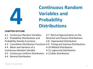
3. Distributions • Important probability distributions • Binominal distribution • Poisson distribution • Gaussian distribution • Cauchy (Breit-Wigner) distribution • Chi-squared distribution • Landau distribution • Uniform distribution • Central limit theorem
3. Distributions 3.1 Binomial distribution Binomial distribution appears when one has exactly two possible trial outcomes (success-failure, head-tail, even-odd, …) event “success”: event “failure”: Probability: Example: (ideal) coins Probability for “head” (A) = p = 0.5, q=0.5 Probability for n=4 trials to get k-time “head” (A) ? k=0: P = (1-p)4 = 1/16 k=1: P = (p (1-p)3) times number of combinations (HTTT, THTT, TTHT, TTTH) = 4*1/16 = ¼ k=2: P = (p2 (1-p)2) times (HHTT, HTTH, TTHH, HTHT, THTH, THHT) = 6*1/16 = 3/8 k=3: P = (p3 (1-p)) times (HHHT, HHTH, HTHH, THHH) = 4*1/15 = ¼ k=4: P = p4 = 1/16 P(0)+P(1)+P(2)+P(3)+P(4) = 1/16+1/4+3/8+1/4+1/16 = 1 ok
3. Distributions 3.1 Binomial distribution • Number of permutations for k successes by n trials: • Binominal coefficient: • Binomial distribution: • Discrete probability distribution • Random variable: k • Depends on 2 parameters: n (number of attempts) and p (probability of suc.) • Sequence of appearance of k successes play no role • - n trials must be independent
3. Distributions 3.1 Binomial distribution (properties) Normalisation: Expectation value (mean value): Proof:
3. Distributions 3.1 Binomial distribution (properties) Variance: Proof: However:
μ x x x x x x x x x x x 3. Distributions 3.1 Binomial distribution HERA-B experiment muon spectrometer 12 chambers; efficiency of one chamber is ε = 95% Trigger condition: 11 out of 12 chambers hit εTOTAL = P(11; 12,0.95) + P(12; 12,0.95) = 88.2 % When chambers reach only ε = 90% then εTOTAL = 65.9% When one chambers fails: εTOTAL = P(11, 0.95, 12) = 56.9 % Random coincidences (noise): εBG = 10% 20% - twice more noise εTOTAL_BG = 1•10-9 2•10-7 200x more background
3. Distributions 3.1 Binomial distribution Example: number of error bars in 1-interval (p=0.68)