Download
1 / 15
190 likes | 617 Views
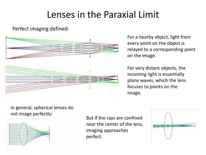
Lenses in the Paraxial Limit. Perfect imaging defined:. For a nearby object, light from every point on the object is relayed to a corresponding point on the image. For very distant objects, the incoming light is essentially plane waves, which the lens focuses to points on the image.

E N D
Lenses in the Paraxial Limit Perfect imaging defined: For a nearby object, light from every point on the object is relayed to a corresponding point on the image. For very distant objects, the incoming light is essentially plane waves, which the lens focuses to points on the image. In general, spherical lenses do not image perfectly: But if the rays are confined near the center of the lens, imaging approaches perfect.
The Paraxial Approximation Using the “sag” form of the conic surface … … and the Taylor Expansion about the origin… We get: The “Paraxial Approximation” will be defined as the region close enough to the Z-axis (r is small enough) such that the surface is accurately described as:
The Effect of a Lens on a Wave in the Paraxial Approximation Consider a thin lens in the paraxial region, with surface curvatures and a plane wave incident on its left side: f Note: The effect of the lens on an incident plane wave is to delay the wave by (n-1)t, where n is the lens’ index of refraction (and assuming the surrounding material is of index n=1), and (where t0 is the thickness at the Z-axis.) Just to the right of the lens the total delay w.r.t. the wave’s vertex is: Which we recognize as a paraxial sphere with curvature The emerging wave therefore converges to a point 1/C past the lens. This, we call the ‘focal length’, f, of the lens.
The “focal length” of a lens is the distance from the lens, f, that a plane wave will be focused to a point. We define the “power” of a lens as: From the previous calculation, we see that the power of a thin lens (in the paraxial approximation) is: This is the “thin lens” equation. We can also see, from the calculation of the wave delay caused by a lens, that a lens of power K will simply add curvature K to the curvature of any incoming wave. K i Consider a wave diverging from point ‘o’, passing a lens of power ‘K’, and converging to point ‘I’: o At the lens, the incoming wave has curvature 1/o, the lens adds curvature K, and the outgoing wave has curvature 1/i. Hence , or: This is the “Imaging Equation”
Paraxial Ray Tracing Although we have derived some basic imaging equations using only the paraxial approximation and the wave nature of light (without even invoking Snell’s Law), the ray approximation will be more useful than wave analysis for analyzing most real optical systems, so we will look at rays in the paraxial approximation. Expanding sin(θ) about zero gives: As a consequence of staying in the region where the spherical surfaces are well approximated by the first term in the Taylor expansion, the ray angles will also all be small, so we can likewise approximate the sin with the first Taylor term, , so Snell’s Law becomes: Additional paraxial assumptions we will use are: For calculating distances, surface sag is ignored as negligible. Angles ≈ sines ≈ tangents
Paraxial Ray Trace through a Surface – Variable Definitions: Angles of incidence and refraction: Ray angles with the Z-axis: Snell’s Law in the Paraxial Approx:
Paraxial Ray Trace Equations: Imaging Since we don’t want to keep calculating angles of incidence and refraction all the time, we will eliminate those angles from Snell’s Law. There are two paths we can take: First, we will eliminate all ray angles and only track object and image distances (the ray intercepts with the Z-axis). Hence The Gaussian surface imaging equation
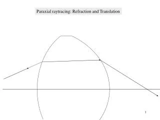
Paraxial Ray Trace Equations: Refraction and Transfer When tracing rays through multiple lens systems, it is often more convenient to keep track of a ray’s angles and height (h,u, u’) rather than its Z-axis intercept points (l,l’). Starting with Snell’s Law and eliminating references to the intercept distances, we get: Hence The Gaussian Refraction Equation for a surface whose power is defined as:
Tracing Through Multiple Lenses In order to trace either rays or images through multiple lenses (or surfaces), we need transfer equations which calculate the input to the next lens from the output of the previous lens. Lens1 Lens2 l2 h1 l’2 u1 u’1 u2 u’2 l1 h2 l’1 For rays, the input angle of a surface is simply the output angle of the previous surface: d1 For the imaging equation, the output image distance for surface i, adjusted by the distance between surfaces, becomes the input object distance for surface i+1: For the refraction equation, the output height modified by the output slope times d gives the input height for the next surface:
Summary of Paraxial Ray Trace Equations This assumes the index before and after the lens = 1 Imaging through a thin lens: Image transfer between lenses: Also assumes the index before and after the lens = 1 Refraction of a ray through a thin lens: Ray transfer between lenses:
Using Gaussian ray traces to generate lens formulas: Trace a horizontal, ray through two lenses (why a horizontal ray?): Location of equivalent lens: The goal is to find the equivalent focal length for the combination of two lenses. The equivalent focal length is defined as the focal length of a single (perfect) lens that would produce the same image.
Ray trace through lens pair: Refract through first element: Refract at second element: Transfer to second element: Eliminating h1 and using where K is the equivalent power of the combination, we get: General formula for combination of two surfaces:
For two lenses in air, spaced by d, then the indices after and between the lenses is n=1, so the two lens formula becomes: Suppose that K1 = 1/d1: What is the power of the combination then?
“Graphical Ray Tracing” Through Thin Lenses We will assume, without further proof, that the paraxial effect of a thin lens on the curvature of wavefronts is, to first order, unchanged by tilting the lens through a “paraxial” angle. Given this, there are a number of rays that can be immediately traced through a thin lens, whose power is known, without further calculation: Incident rays parallel to the axis, pass through the focal point. (The corollary is that incident rays that pass through the focal point emerge parallel to the axis.) Rays through the center of the lens are undeviated. In the paraxial approximation, the lens is an infinitesimally thin plane-parallel plate at the center. Any parallel bundle of rays will meet at the focal plane at the point where the central (undeviated) ray in the bundle meets that plane. The “focal plane” is a plane perpendicular to the axis at the focal distance. The central ray of a bundle is often called the “chief ray”. For object and image distances determined by the thin lens imaging equation, a bundle of rays diverging from any point on the object plane will converge to a point on the image plane at the point where the chief ray from the object point intersects the image plane.