Download
1 / 87
870 likes | 1k Views
This presentation, held on June 6, 2002, at IIS Sinica, explores key approximation algorithms for scheduling problems involving average completion time. It covers non-preemptive scheduling on single and parallel machines with precedence constraints, focusing on achieving optimal solutions and approximation bounds. The discussion includes techniques such as Shortest Job First (SJF), linear programming, and various approximation algorithms for single-machine and m-machine problems. Attendees will gain insights into the complexities of these scheduling challenges and the related research findings.

E N D
Approximation Techniques for Average Completion Time Scheduling 報告人:羅習五, 魏仲佑, 陳雅淑, 姜柏任, 陳建佳 時間:June 6, 2002, Thursday, 4pm 地點:, IIS, Sinica, Room 724)
目標: • 介紹所有待會用到的演算法基礎 • 說明與內容息息相關的相關研究 • 因為時間關係,不詳細說明相關研究的成果 • 希望能讓大家先以直關的方式去思考這些演算法
Introduction • 這篇論文所要談論的是non-preemptive的排程問題 • Single machine的問題 • Parallel machine的問題 • 含有precedence的問題 • 底下我們先約略的探討這些問題的難度
One machine problem • 給n個task每個task都有自己的release time, processing time及weight,請問該如何排程才可以使得average weighted completion time最小 • 假設release time都為0 • 優先執行(processing time / weight)最小的task • P的時間就可以得到optimal solution • 假設是preemptive • 使用SJF (shortest job first)即可 • P的時間就可以得到optimal solution • 待會會把這個當成是optimal solution的Lower bound
One machine problem • 放寬限制一:假設可搶先 • 先使用SJF跑一遍然後得到所有task在此狀況下的complete time, 然後再依照completion time的順序執行所有的task • 2-approximation (worst case) • 是所有以知的deterministic on-line algorithm中最好的 • 放寬限制二:linear programming • 放寬限制三:假設可搶先並且所有的task的processing time乘上一個介於0~1間的值 • 同上,利用completion time的順序執行所有task • 明顯的,如果乘上不一樣的值會有不一樣的結果參數化
獲致的結果 • Deterministic off-line algorithm • 1.58 – approximation • Optimal randomized on-line algorithm • 1.58 – approximation
m-Machine Problem • 問題和single-machine problem類似,只是現在總共有m個machine可供使用 • 該如何定義”好” • Optimal solution的lower bound為何 • 是否可以定義preempt版本的m-Machine problem的optimal solution為lower bound • 可搶先版的問題也是NP-Hard • 如果定義為前者的話,那麼我們的演算法可以有多好 • 其實也不能保證到多好
放寬限制 • 改成可搶先 • 14/3-approximation • 改成linear programming • 24-approximation • 4-(1/m)-approximation • 3.5-approximation • 改成可搶先,並且processing time = processing time/m • 3-approximation
Scheduling with precedence constrain • 問題和之前的差不多,只不過各個task之間已經不再是independent的關係
困難度 • Single machine的狀況 • Without release dates NP-hard • 2-approximation • With release dates • 2.718-approximation • m-Machine的狀況 • Without release dates & precedence constrain NP-hard • Without weights and precedence graph is union of chain NP-hard
One-machine Scheduling • Input: A process sets P = {p1, p2, ……,pn} with computation time {c1, c2, ……, cn} and release dates {d1, d2, ……, dn} • Output: minimized the average completion time of the process set in one machine. • Fact: • 1. P if process sets are preemptive. (shortest remaining processing time first, SRPT) • 2. P if release dates are all 0. • 3. Otherwise, NP-hard.
One-machine Scheduling cont. • 2-approximation was proposed by Phllips, Stein, and Wein: • An optimal preemptive schedule P is found with SRPT algorithm. • Given P, the jobs are ordered by increasing completion times, CiP, it is clear that this algorithm is 2-approximation (prove later) • The authors in this paper extend the idea above and proposed a new algorithm called -algorithm.
Algorithm • Algorithm: • Given a preemptive schedule P and (0, 1], define CjP() to be the time at which pj, an fraction of Jj, is completed. • Execute the process according to the sorted CjP() • Clearly, an algorithm is either on-line or off-line. • Observation: • 1. The algorithm is either on-line or off-line • 2.if = 1, this algorithm is the same as previous algorithm.
Algorithm cont. • Approximation analysis: • 1. Is it P? • 2. Is it feasible? • 3. It’s approximation ration? 1+1/, will prove later. • 4. Tight? Yes • The weighted version doesn’t improved. • Fact:4/3 approximation with preemptive algo. • Fact:2.12 for non-preemptive algo.
One-machine scheduling with release dates • Let P be a preemptive schedule, and denote the completion time of Ji in P and in the nonpreemptive -schedule derived from P, respectively • Theorem 2.1: Given an instance of one-machine scheduling with release dates, for any (0,1], an -schedule has further, there are instances where the inequality is asymptotically tight.
Proof of Theorem 2.1(1/2) • index the jobs by the order of their -points in the preemptive schedule P. • let be the latest release date among jobs with points no greater than j’s • By time , jobs 1 through j have all been released, hence ………………(2.1)
Proof of Theorem 2.1(2/2) • ,since only an fraction j has finished by • , since fractions of job 1,..,j must run before time • (2.1)
Tightness of theorem 2.1 x jobs P0=1 P1= P2=...=Px+1 = 0 0 - + 1 1+ 1+ points: P0 P1 P0 P0 Optimal: +x(+)+(1+) P2...Px+1 P2...Px+1 P1 P0 schedule: +(1+)+x(1+ ) as x>>1, ->0, ratio ->
more about theorem 2.1 • since (0,1], this theorem yields approximation bounds that are worse than 2. • However, we will introduce a new fact that ultimately yield better algorithms that makespan of an -schedule is within a (1+ )-factor of the makespane of the corresponding preemptive schedule.
more about theorem 2.1 • The idle time introduced in the nonpreemptive schedules decrease as is reduced from 1 to 0. • The (worst-case) bound on the completion time of any specific job increase as goest from 1 to 0. • It is the balancing of these two effects that leads to better approximations.
refinement of theorem 2.1 • Let denote the set of jobs which complete exactly fraction of their processing time before in the schedule P, P is a preemptive schedule. (Ji is included in ). • we also overload to denote the sum of processing times of all jobs in the set • Let Ti be the total idle time in P before Ji completes.
refinement of theorem 2.1 • Preemptive completion time of Ji can be written as the sum of the idle time and fractional processing times of jobs that ran before . • lemma2.2 We next upper bound the completion time of a job Ji in the -schedule. • lemma 2.3
proof of lemma 2.3 • Let J1,...,Ji-1 be the jobs that run before Ji in the -schedule. We will give a procedure whcich converts the preemptive schedule into a schedule in which (C1) jobs J1,...,Ji run nonpreemptively in that order (C2) the remaining jobs run preemptively, and (C3) the completion time of Ji obeys the bound given in the lemma 2.2
proof of lemma 2.3 • splitting the 2nd term in the lemma 2.2 (1) (2) (3) (4)
proof of lemma 2.3 • Let JB = and JA = J – JB • the idle time in the preemptive schedule before • the pieces of jobs in JA hat ran before • for each job Jj JB, the pieces of Jj that ran before • for each job Jj JB, the pieces of Jj that ran between and
proof of lemma 2.3 • Let xj be the for which Jj ,that is, the fraction of Jj that was completed before • (xj - )pj is the fraction of job Jj that ran between and
proof of lemma 2.3 • Let JC = {J1,...,Ji}, the jobs that run no later than Ji in -schedule. • Thus, JC JB • Now, think of schedule P as an ordered list of pieces of jobs (with size).
proof of lemma 2.3 • for each Jj JC modify the list by • 1. removing all pieces of jobs that run between and • 2.inserting a piece of size (xj - )pj at point corresponding to • now, we have pieces of size (xj - )pj of jobs j1,...ji in the correct order (plus other pieces of jobs) • convert this ordered list back into a schedule by scheduling the pieces in the order of the list, respecting release dates. • claim that ji still completes at time
Example: =1/2, i = 4 time 0 Job1 Job2 SRPT schedule and ½ completion times Job3 Job4 after 1. 2. schedule by release dates
proof of lemma 2.3 • the total processing time before remains unchanged and that other than the pieces of size (xj - )pj , we moved pieces only later in time, so no additional idle time need be introduced. • for each job Jj JC, extend the piece of size (xj - )pj to one of size pj by adding pj - (xj-)pj units of processing and replace the pieces of Jj that occur earlier, of total size pj, by idle time.
Example: =1/2, i = 4 time 0 Job1 Job2 SRPT schedule and ½ completion times Job3 Job4 extending the pieces to complete the schedule used in the proof the true ½-schedule
proof of lemma 2.3 • the completion time of Ji is ...........reindexing j by ..........lemma 2.2
proof of lemma 2.3 • To complete the proof, observe that the remaining pieces in the schedule are all from jobs in J- JC, and we have thus met the conditions (C1),(C2),(C3) above. • applying lemma 2.3 to the last job to complete in the -schedule yields the corollary 2.4
corollary 2.4 • The makespan of the -schedule is at most (1+ ) times the makespan of the corresponding preemptive schedule, and there are instances for which this bound is tight.
Random- Algorithm • Observation: a key observation is that a worse-case instance that induces a performance ration 1+1/ is not a worse-case instance for many other values of . • The previous observation suggests the authors to develop a randomized algorithm to pick randomly. • The authors propose on-line algorithm with expected 1/(e-1) approximation and off-line algorithm with 1/(e-1) approximation.
Random- Algorithm cont. • According to previous lemma, the approximation ratio is going to depend on the distribution of the different sets SiP(). • To avoid the worse case , we choose randomly according to some probability distribution. • Lemma 2.5: suppose is chosen from a probability distribution over (0, 1] with a density function f. Then for each job Ji, E[Ci] (1+) CiP. It follows that E[iCi] i(1+) CiP.
Random- Algorithm cont. • From lemma 2.3: • Therefore:
Random- Algorithm cont. • According to lemma 2.2 and lemma 2.5, it follows that • Using linearity of expectations, the expected total completion time of schedule is within (1+) of the preemptive schedule’s total completion time.
Random- Algorithm cont. • For the problem of scheduling to minimize weighted completion time with release dates, Random- performs as follows: • (1) If is chosen uniformly in (0, 1], the expected approximation ratio is at most 2 • (2) If is chosen to be 1 with probability 3/5 and ½ with probability 2/5, the expected approximation ratio is at most 1.8 • (3) If is chosen from (0, 1] according to the density function f() = e/(e-1), the expected approximation ratio is at most e/(e-1) 1.58
Random- Algorithm cont. • Proof of (1): choosing uniformly corresponds to the f() = 1, according to lemma 2.5, the we get an approximation ratio of 2.
Random- Algorithm cont. • Proof of (3)
Random- Algorithm cont. • =1/e-1 • 1+1/(e-1) e/(e-1) • Proof of (2): omitted • The density function e/(e-1) minimize over all choices of f().
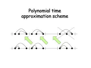
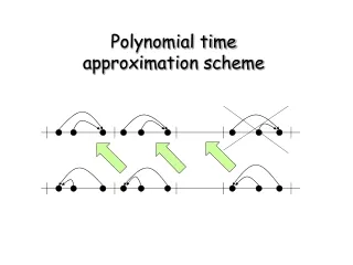
Best- Algorithm • In the off-line setting, rather than choosing randomly, we can try different values of and choose the one that yields the best schedule. This is called Best- scheduling. • Corollary: Algorithm Best- is an e/(e-1)-approximation algorithm for non-preemptive scheduling to minimize average completion time on one machine with release dates. It runs O(n2) time.
Best- Algorithm cont. • Approximation ratio follows from previous theorem. • The SRPT schedule preempts only at release dates so that it has at most n-1 preemptions and there are at most n combinatorially distinct value of for a given preemptive schedule. • The SRPT schedule can be computed in O(nlogn) time using a simple priority queue and given the schedule and an . The corresponding -schedule can be computed in linear time by a simple scan.
On-line Random- Scheduling • Theorem: There is a polynomial-time randomized on-line algorithm with an expected competitive ratio e/(e-1) for the problem of minimizing total completion time in the presence of release dates. • The algorithm picks an (0,1] according to the density function f(x) = ex/(e-1) before receiving any input. • The algorithm simulates the on-line preemptive SRPT schedule. At the exact time when a job finishes a fraction of its processing time in the simulated SRPT schedule, it is added to the queue of jobs to be executed non-preemptively.
On-line Random- Scheduling cont. • The non-preemptive schedule is obtained by executing jobs in the strict order in the queue. • This is a valid on-line scheduling. • The bound on the expected competitive ratio is the same as theorem 2.6. Since lemma 2.3 does not apply the true schedule, but a weaker one in which for every job Ji the first fraction of its processing time in the SRPT schedule is left as idle time.
Negative Results • There are negative results for the various algorithm • 1. If is chosen uniformly, the expected approximation ratio is at least 2 • 2. For the Best- algorithm, the approximation ratio is at least 4/3