Download

1 / 25
250 likes | 411 Views
Alignment methods. April 26, 2011 Return Quiz 1 today Return homework #4 today. Next homework due Tues, May 3 Learning objectives- Understand the Smith-Waterman algorithm. Have a general understanding about PAM and BLOSUM scoring matrices. Workshop-Compare scoring matrices.

E N D
Alignment methods • April 26, 2011 • Return Quiz 1 today • Return homework #4 today. • Next homework due Tues, May 3 • Learning objectives- Understand the Smith-Waterman algorithm. Have a general understanding about PAM and BLOSUM scoring matrices. • Workshop-Compare scoring matrices.
Smith-Waterman Algorithm Advances inApplied Mathematics, 2:482-489 (1981) Smith-Waterman algorithm –can be used for global or local alignment -Memory intensive -Common searching programs such as BLAST use SW algorithm
Smith-Waterman algorithm Mi,j = MAXIMUM [ Mi-1, j-1 + si,,j (match or mismatch in the diagonal), Mi, j-1+ w (gap in sequence #1), Mi-1, j + w (gap in sequence #2), 0] Where Mi-1, j-1 is the value in the cell diagonally juxtaposed to Mi,j. (The i-1, j-1 cell is up and to the left of mi,nj). Where si,j is the value for the match or mismatch in the minj cell. Where Mi, j-1 is the value in the cell above Mi,j. Where w is the value for the gap penalty. Where Mi-1, j is the value in the cell to the left of Mi,j.
Two sequences to align • Sequence 1: ABCNJRQCLCRPM • Sequence 2: AJCJNRCKCRBP
Initialization step: create matrix with M + 1 columns and N + 1 rows. M = number of letters in sequence 1 and N = number of letters in sequence 2. First column (M-1) and first row (N-1) will be filled with 0’s.
Matrix fill step: Each position Mi,j is defined to be the MAXIMUM score at position i,j Mi,j = MAXIMUM [ Mi-1, j-1 + si,,j (match or mismatch in the diagonal) Mi, j-1 + w (gap in sequence #1) Mi-1, j + w (gap in sequence #2)] row column
Sequence 1: ABCNJ-RQCLCR-PM Sequence 2: AJC-JNR-CKCRBP- Score : 8
Smith-Waterman (local alignment) a. Initializes edges of the matrix with zeros b. It searches for sequence matches. c. Assigns a score to each pair of amino acids -uses similarity scores -uses positive scores for related residues -uses negative scores for substitutions and gaps d. Scores are summed for placement into Mi,j. If any sum result is below 0, a 0 is placed into Mi,j. e. Backtracing begins at the maximum value found anywhere in the matrix. f. Backtrace continues until the it meets an Mi,j value of 0.
A W G H E A W – H E Score: 5 15 -8 10 6 Total score: 28 Pecent similarity: 4/5 x 100 = 80%
How does one achieve the “perfect database search”? • Consider the following: • Scoring Matrices (PAM vs. BLOSUM) • Local alignment algorithm • Database • Search Parameters • Expect Value-change threshold for score reporting • Filtering-remove repeat sequences
PAM-1 BLOSUM-100 Small evolutionary distance High identity within short sequences Which Scoring Matrix to use? • PAM-250 • BLOSUM-20 • Large evolutionary distance • Low identity within long sequences
BLOSUM Scoring Matrices Which BLOSUM Matrix to use? BLOSUM Identity (up to) 80 80% 62 62% (usually default value) 35 35% If you are comparing sequences that are very similar, use BLOSUM 80. Sequences that are more divergent (dissimilar) than 20% are given very low scores in this matrix.
Replacement amino acid Original amino acid
Figure 4.2 Numbers of accepted point mutations (multiplied by 10). A total of 1572 exchanges are shown. Positions with red dashes are Mjj values. Modified from Dayhoff, 1978.
Relative mutability calculations Figure 4.3 Simplified example to show how relative mutability is calculated.
Development of the Mutation Probability Matrix. (2) Figure 4.4. Mutational Probability Matrix (partial). This only shows 5 of the 20 amino acids in the MPM. Numbers were multiplied by 10,000 to make it easier to read. The numbers for each column adds up to 10,000. In the top row there are the replacement amino acids a nd on the left column are the original amino acids. Mjj values shown are 9867, 9913, 9822, 9859 and 9973.
What is percent of amino acids that differ in the MPM? This value totals 99 for each amino acid. There is a 1% difference for each amino acid
Conversion of the PAM1 Mutational Probability Matrix to the PAM1 Scoring Matrix.
Conversion of the PAM1 Mutational Probability Matrix to other PAM scoring matrices. 1Mutation Probability Matrices generated by the equation (PAM1 MPM)n where n is the number listed in the first column.