Download

1 / 38
390 likes | 543 Views
fMRI design and analysis. Advanced designs. (Epoch) fMRI example…. =. b 1. +. b 2. voxel timeseries. box-car function. baseline (mean). + (t). (box-car unconvolved). (Epoch) fMRI example…. data vector (voxel time series). parameters. error vector. design matrix. b 1.

E N D
fMRI design and analysis Advanced designs
(Epoch) fMRI example… = b1 + b2 voxel timeseries box-car function baseline (mean) + (t) (box-car unconvolved)
(Epoch) fMRI example… data vector (voxel time series) parameters error vector design matrix b1 = + b2 y = X +
(Epoch) fMRI example……fitted and adjusted data Raw fMRI timeseries Adjusted data fitted box-car highpass filtered (and scaled) Residuals fitted high-pass filter
Convolution with HRF Unconvolved fit Residuals = Boxcar function convolved with HRF hæmodynamic response Convolved fit Residuals (less structure)
Fixed vs. Random Effects Multi-subject Fixed Effect model Subject 1 error df ~ 300 Subject 2 Subject 3 Subject 4 Subject 5 Subject 6 • Subjects can be Fixed or Random variables • If subjects are a Fixed variable in a single design matrix (SPM “sessions”), the error term conflates within- and between-subject variance • But in fMRI (unlike PET) the between-scan variance is normally much smaller than the between-subject variance • If one wishes to make an inference from a subject sample to the population, one needs to treat subjects as a Random variable, and needs a proper mixture of within- and between-subject variance • In SPM, this is achieved by a two-stage procedure: • 1) (Contrasts of) parameters are estimated from a (Fixed Effect) model for each subject • 2) Images of these contrasts become the data for a second design matrix (usually simple t-test or ANOVA)
Two-stage “Summary Statistic” approach 1st-level (within-subject) 2nd-level (between-subject) One-sample t-test ^ (1) N=6 subjects (error df =5) ^ b1 ^ (2) ^ b2 contrast images of cbi ^ (3) ^ b3 p < 0.001 (uncorrected) ^ (4) ^ SPM{t} b4 ^ bpop ^ (5) ^ b5 WHEN special case of n independent observations per subject: var(bpop) = 2b/ N + 2w / Nn ^ (6) ^ b6 ^ w= within-subject error
Types of Errors Is the region truly active? Yes No Type I Error HIT Yes Does our stat test indicate that the region is active? Type II Error Correct Rejection No p value: probability of a Type I error e.g., p <.05 “There is less than a 5% probability that a voxel our stats have declared as “active” is in reality NOT active Slide modified from Duke course
Multiple comparisons… SPM{t} Eg random noise pu = 0.05 Gaussian10mm FWHM (2mm pixels) • If n=100,000voxels tested with pu=0.05 of falsely rejecting Ho... • …then approx n pu (eg 5,000) will do so by chance (false positives, or “type I” errors) • Therefore need to “correct” p-values for number of comparisons • A severe correction would be a Bonferroni, where pc = pu/n… • …but this is only appropriate when the n tests independent… • … SPMs are smooth, meaning that nearby voxels are correlated • => Random Field Theory...
Consider SPM as lattice representation of continuous random field “Euler characteristic”: a topological measure (# “components” - # “holes”) Euler depends on smoothness Smoothness estimated by covariance of partial derivatives of residuals (expressed as “resels” or FWHM) Smoothness does not have to be stationary (for height thresholding): estimated locally as “resels-per-voxel” (RPV) Random Field Theory (RFT)
Design Types = trial of one type (e.g., face image) = null trial (nothing happens) = trial of another type (e.g., place image) Block Design Slow ER Design Rapid Counterbalanced ER Design Rapid Jittered ER Design Mixed Design
An Example Culham et al., 1998, J. Neuorphysiol.
Analysis of Parametric Designs parametric variant: passive viewing and tracking of 1, 2, 3, 4 or 5 balls
Factorial Designs Example: Sugiura et al. (2005, JOCN) showed subjects pictures of objects and places. The objects and places were either familiar (e.g., the subject’s office or the subject’s bag) or unfamiliar (e.g., a stranger’s office or a stranger’s bag) This is a “2 x 2 factorial design” (2 stimuli x 2 familiarity levels)
Statistical Approaches In a 2 x 2 design, you can make up to six comparisons between pairs of conditions (A1 vs. A2, B1 vs. B2, A1 vs. B1, A2 vs. B2, A1 vs. B2, A2 vs. B1). This is a lot of comparisons (and if you do six comparisons with p < .05, your overall p value is .05 x 6 = .3 which is high). How do you decide which to perform?
Factorial Designs Main effects Difference between columns Difference between rows Interactions Difference between columns depending on status of row (or vice versa)
Main Effect of Stimuli In LO, there is a greater activation to Objects than Places In the PPA, there is greater activation to Places than Objects
Main Effect of Familiarity In the precuneus, familiar objects generated more activation than unfamiliar objects
Interaction of Stimuli and Familiarity In the posterior cingulate, familiarity made a difference for places but not objects
Using fMR Adaptation to Study Coding Example: We know that neurons in the brain can be tuned for individual faces “Jennifer Aniston” neuron in human medial temporal lobe Quiroga et al., 2005, Nature
Using fMR Adaptation to Study Tuning Activation Activation Activation Activation • fMRI resolution is typically around 3 x 3 x 6 mm so each sample comes from millions of neurons Neuron 1 likes Jennifer Aniston Neuron 2 likes Julia Roberts Neuron 3 likes Brad Pitt Even though there are neurons tuned to each object, the population as a whole shows no preference
fMR Adaptation If you show a stimulus twice in a row, you get a reduced response the second time Hypothetical Activity in Face-Selective Area (e.g., FFA) Unrepeated Face Trial Activation Repeated Face Trial Time
fMRI Adaptation “different” trial: 500-1000 msec “same” trial: Slide modified from Russell Epstein
Viewpoint dependence in LOC LO pFs (~=FFA) Source: Kalanit Grill-Spector
Adaptation to speaker identity • fMRI adaptation • 14 subjects, passive listening • 12 ‘adapt-Syllable’ blocs • (1 syllable, 12 speakers) • 12 ‘adapt-Speaker’ blocs • (1 speaker, 12 words) • Same 144 stimuli in the two conditions Belin & Zatorre (2003) Neuroreport
Petkov et al (2008) Nat Neurosci Adaptation to speaker identity Belin & Zatorre (2003) Neuroreport Von Kriegstein et al (2003) Cognitive Brain Research
Problems The basis for effect is not well-understood this is seen in the many terms used to describe it • fMR adaptation (fMR-A) • priming • repetition suppression The effect could be due to many factors such as: repeated stimuli are processed more “efficiently” • more quickly? • with fewer action potentials? • with fewer neurons involved? repeated stimuli draw less attention repeated stimuli may not have to be encoded into memory repeated stimuli affect other levels of processing with input to area demonstrating adaptation (data from Vogels et al.) subjects may come to expect repetitions and their predictions may be violated by novel stimuli (Summerfield et al., 2008, Nat. Neurosci.)
Multivariate statistics Traditional fMRI analyses use a ‘massive univariate approach’ -> Information on the sensitivity of brain regions to sensory stimulation or cognitive tasks But they miss the potentially rich information contained in the pattern ofdistributed activity over a number of voxels.
Data Driven Analyses Hasson et al. (2004, Science) showed subjects clips from a movie and found voxels which showed significant time correlations between subjects
Reverse correlation They went back to the movie clips to find the common feature that may have been driving the intersubject consistency