Download
1 / 16
160 likes | 338 Views
Survey of gradient based constrained optimization algorithms. Select algorithms based on their popularity. Additional details and additional algorithms in Chapter 5 of Haftka and Gurdal’s Elements of Structural Optimization. Optimization with constraints. Standard formulation

E N D
Survey of gradient based constrained optimization algorithms • Select algorithms based on their popularity. • Additional details and additional algorithms in Chapter 5 of Haftka and Gurdal’s Elements of Structural Optimization
Optimization with constraints • Standard formulation • Equality constraints are a challenge, but are fortunately missing in most engineering design problems, so this lecture will deal only with equality constraints.
Derivative based optimizers • All are predicated on the assumption that function evaluations are expensive and gradients can be calculated. • Similar to a person put at night on a hill and directed to find the lowest point in an adjacent valley using a flashlight with limited battery • Basic strategy: • Flash light to get derivative and select direction. • Go straight in that direction until you start going up or hit constraint. • Repeat until converged. • Some methods move mostly along the constraint boundaries, some mostly on the inside (interior point algorithms)
Gradient projection and reduced gradient methods • Find good direction tangent to active constraints • Move a distance and then restore to constraint boundaries • A typical active set algorithm, used in Excel
Penalty function methods • Quadratic penalty function • Gradual rise of penalty parameter leads to sequence of unconstrained minimization technique (SUMT). Why is it important?
Contours for r=1000 . For non-derivative methods can avoid this by having penalty proportional to absolute value of violation instead of its square!
Problems Penalty • Find how many function evaluatonsfminuncand fminsearch solve Example 5.7.1 when you use r=1000 starting from x0=[2,2]. • Compare to going through r=1,10,100,1000, and starting the solution for the next r value where the solution for the previous one stopped.
5.9: Projected Lagrangian methods • Sequential quadratic programming • Find direction by solving • Find alpha by minimizing
Matlab function fmincon FMINCON attempts to solve problems of the form: min F(X) subject to: A*X <= B, Aeq*X = Beq (linear cons) X C(X) <= 0, Ceq(X) = 0 (nonlinear cons) LB <= X <= UB [X,FVAL,EXITFLAG,OUTPUT,LAMBDA] =FMINCON(FUN,X0,A,B,Aeq,Beq,LB,UB,NONLCON) The function NONLCON accepts X and returns the vectors C and Ceq, representing the nonlinear inequalities and equalities respectively. (Set LB=[] and/or UB=[] if no bounds exist.) . Possible values of EXITFLAG 1 First order optimality conditions satisfied. 0 Too many function evaluations or iterations. -1 Stopped by output/plot function. -2 No feasible point found.
Quadratic function and constraintexample function f=quad2(x) Global a f=x(1)^2+a*x(2)^2; end function [c,ceq]=ring(x) global riro c(1)=ri^2-x(1)^2-x(2)^2; c(2)=x(1)^2+x(2)^2-ro^2; ceq=[]; end x0=[1,10];a=10;ri=10.; ro=20; [x,fval]=fmincon(@quad2,x0,[],[],[],[],[],[],@ring) x =10.0000 -0.0000 fval =100.0000
Fuller output [x,fval,flag,output,lambda]=fmincon(@quad2,x0,[],[],[],[],[],[],@ring) Optimization completed because the objective function is non-decreasing in feasible directions, to within the default value of the function tolerance, and constraints are satisfied to within the default value of the constraint tolerance. x =10.0000 -0.0000 fval =100.0000 flag = 1 output = iterations: 6 funcCount: 22 lssteplength: 1 stepsize: 9.0738e-06 algorithm: 'medium-scale: SQP, Quasi-Newton, line-search' firstorderopt: 9.7360e-08 constrviolation: -8.2680e-11 lambda.ineqnonlin’=1.0000 0
Making it harder for fmincon a=1.1; [x,fval,flag,output,lambda]=fmincon(@quad2,x0,[],[],[],[],[],[],@ring) Maximum number of function evaluations exceeded; increase OPTIONS.MaxFunEvals. x =4.6355 8.9430 fval=109.4628 flag=0 iterations: 14 funcCount: 202 lssteplength: 9.7656e-04 stepsize: 2.2830 algorithm: 'medium-scale: SQP, Quasi-Newton, line-search' firstorderopt: 5.7174 constrviolation: -6.6754
Restart sometimes helps x0=x x0 = 4.6355 8.9430 [x,fval,flag,output,lambda]=fmincon(@quad2,x0,[],[],[],[],[],[],@ring) x =10.0000 0.0000 fval=100.0000 flag = 1 iterations: 15 funcCount: 108 lssteplength: 1 stepsize: 4.6293e-04 algorithm: 'medium-scale: SQP, Quasi-Newton, line-search' firstorderopt: 2.2765e-07 constrviolation: -2.1443e-07
Problem fmincon • For the ring problem with a=10, find how the number of function evaluations depends on how narrow you can make the ring (by reducing ro). Always start with x0=[1,10]