Download

1 / 167
1.69k likes | 1.85k Views
Chapter 12 Software Optimisation. Software Optimisation Chapter. This chapter consists of three parts: Part 1: Optimisation Methods. Part 2: Software Pipelining. Part 3: Multi-cycle Loop Pipelining. Chapter 12 Software Optimisation Part 1 - Optimisation Methods. Objectives.

E N D
Chapter 12 Software Optimisation
Software Optimisation Chapter This chapter consists of three parts: Part 1: Optimisation Methods. Part 2: Software Pipelining. Part 3: Multi-cycle Loop Pipelining.
Chapter 12 Software Optimisation Part 1 - Optimisation Methods
Objectives • Introduction to optimisation and optimisation procedure. • Optimisation of C code using the code generation tools. • Optimisation of assembly code.
Introduction • Software optimisation is the process of manipulating software code to achieve two main goals: • Faster execution time. • Small code size. Note: It will be shown that in general there is a trade off between faster execution type and smaller code size.
Introduction • To implement efficient software, the programmer must be familiar with: • Processor architecture. • Programming language (C, assembly or linear assembly). • The code generation tools (compiler, assembler and linker).
Optimising C Compiler Options • The ‘C6x optimising C compiler usesthe ANSI C source code and can perform optimisation currently up-to about 80% compared with a hand-scheduled assembly. • However, to achieve this level of optimisation, knowledge of different levels of optimisation is essential. Optimisation is performed at different stages and levels.
Assembly Optimisation • To develop an appreciation of how to optimise code, let us optimise an FIR filter: • For simplicity we write: [1]
Assembly Optimisation • To implement Equation 1, we need to perform the following steps: (1) Load the sample x[i]. (2) Load the coefficients h[i]. (3) Multiply x[i] and h[i]. (4) Add (x[i] * h[i]) to the content of an accumulator. (5) Repeat steps 1 to 4 N-1 times. (6) Store the value in the accumulator to y.
Assembly Optimisation MVK .S1 0,B0 ; Initialise the loop counter MVK .S1 0,A5 ; Initialise the accumulator loop LDH .D1 *A8++,A2 ; Load the samples x[i] LDH .D1 *A9++,A3 ; Load the coefficients h[i] NOP 4 ; Add “nop 4” because the LDH has a latency of 5. MPY .M1 A2,A3,A4 ; Multiply x[i] and h[i] NOP ; Multiply has a latency of 2 cycles ADD .L1 A4,A5,A5 ; Add “x [i]. h[i]” to the accumulator [B0] SUB .L2 B0,1,B0 ; [B0] B .S1 loop ; loop overhead NOP 5 ; The branch has a latency of 6 cycles • Steps 1 to 6 can be translated into the following ‘C6x assembly code:
Assembly Optimisation • In order to optimise the code, we need to: (1) Use instructions in parallel. (2) Remove the NOPs. (3) Remove the loop overhead (remove SUB and B: loop unrolling). (4) Use word access or double-word access instead of byte or half-word access.
Step 1 - Using Parallel Instructions Cycle .D1 .D1 .D2 .D2 .M1 .M2 .L1 .L2 .S1 .S2 NOP 1 2 3 4 5 6 7 8 9 10 11 12 13 14 15 16 ldh ldh nop nop nop nop mpy nop add sub b nop nop nop nop nop
Step 1 - Using Parallel Instructions Cycle .D1 .D1 .D2 .D2 .M1 .M2 .L1 .L2 .S1 .S2 NOP 1 2 3 4 5 6 7 8 9 10 11 12 13 14 15 16 ldh ldh nop nop nop nop mpy nop add sub b nop nop nop Note: Not all instructions can be put in parallel since the result of one unit is used as an input to the following unit. nop nop
Step 2 - Removing the NOPs Cycle .D1 .D1 .D2 .D2 .M1 .M2 .L1 .L2 .S1 .S2 NOP 1 2 3 4 5 6 7 8 9 loop LDH .D1 *A8++,A2 LDH .D1 *A9++,A3 [B0] SUB .L2 B0,1,B0 [B0] B .S1 loop NOP 2 MPY .M1 A2,B3,A4 NOP ADD .L1 A4,A5,A5 10 11 12 13 14 15 16 ldh ldh sub b nop nop mpy nop add
Step 3 - Loop Unrolling LDH .D1 *A8++,A2 ;Start of iteration 1 || LDH .D2 *B9++,B3 NOP 4 MPY .M1X A2,B3,A4 ;Use of cross path NOP ADD .L1 A4,A5,A5 LDH .D1 *A8++,A2 ;Start of iteration 2 || LDH .D2 *B9++,B3 NOP 4 MPY .M1 A2,B3,A4 NOP ADD .L1 A4,A5,A5 ; : ; : ; : LDH .D1 *A8++,A2 ; Start of iteration n || LDH .D2 *B9++,B3 NOP 4 MPY .M1 A2,B3,A4 NOP ADD .L1 A4,A5,A5 loop LDH .D1 *A8++,A2 LDH .D1 *A9++,A3 [B0] SUB .L2 B0,1,B0 [B0] B .S1 loop NOP 2 MPY .M1 A2,A3,A4 NOP ADD .L1 A4,A5,A5 • The SUB and B instructions consume at least two extra cycles per iteration (this is known as branch overhead).
Step 4 - Word or Double Word Access • The ‘C6711 has two 64-bit data buses for data memory access and therefore up to two 64-bit can be loaded into the registers at any time (see Chapter 2). • In addition the ‘C6711 devices have variants of the multiplication instruction to support different operation (see Chapter 2). Note: Store can only be up to 32-bit.
Step 4 - Word or Double Word Access loop LDW .D1 *A9++,A3 ; 32-bit word is loaded in a single cycle || LDW .D2 *B6++,B1 NOP 4 [B0] SUB .L2 [B0] B .S1 loop NOP 2 MPY .M1 A3,B1,A4 || MPYH .M2 A3,B1,B3 NOP ADD .L1 A4,B3,A5 • Using word access, MPY and MPYH the previous code can be written as: • Note: By loading words and using MPY and MPYH instructions the execution time has been halved since in each iteration two 16x16-bit multiplications are performed.
Optimisation Summary • It has been shown that there are four complementary methods for code optimisation: • Using instructions in parallel. • Filling the delay slots with useful code. • Using word or double word load. • Loop unrolling. These increase performance and reduce code size.
Optimisation Summary • It has been shown that there are four complementary methods for code optimisation: • Using instructions in parallel. • Filling the delay slots with useful code. • Using word or double word load. • Loop unrolling. This increases performance but increases code size.
Chapter 12 Software Optimisation Part 2 - Software Pipelining
Objectives • Why using Software Pipelining, SP? • Understand software pipelining concepts. • Use software pipelining procedure. • Code the word-wide software pipelined dot-product routine. • Determine if your pipelined code is more efficient with or without prolog and epilog.
Why using Software Pipelining, SP? • SP creates highly optimized loop-code by: • Putting several instructions in parallel. • Filling delay slots with useful code. • Maximizes functional units. • SP is implemented by simply using the tools: • Compiler options -o2 or -o3. • Assembly Optimizer if .sa file.
Software Pipeline concept LDH || LDH MPY ADD How many cycles wouldit take to perform thisloop 5 times? (Disregard delay-slots). ______________ cycles To explain the concept of software pipelining, we will assume that all instructions execute in one cycle.
Software Pipeline Example LDH || LDH MPY ADD How many cycles wouldit take to perform thisloop 5 times? (Disregard delay-slots). ______________ cycles 5 x 3 = 15 Let’s examine hardware (functional units) usage ...
Non-Pipelined Code Cycle 1 .D1 ldh .D2 ldh .M1 .M2 .L1 .L2 .S1 .S2 2 3 4 ldh ldh 5 mpy 6 add 7 ldh ldh 8 mpy 9 add .D1 .D2 mpy add
Pipelining Code Cycle 1 ldh .D1 ldh .D2 .M1 .M2 .L1 .L2 .S1 .S2 2 ldh ldh mpy 3 ldh ldh mpy add 4 ldh ldh mpy add 5 ldh ldh mpy add 6 mpy add 7 add Pipelining these instructions took 1/2 the cycles!
Pipelining Code Cycle 1 ldh .D1 ldh .D2 .M1 .M2 .L1 .L2 .S1 .S2 2 ldh ldh mpy 3 ldh ldh mpy add 4 ldh ldh mpy add 5 ldh ldh mpy add 6 mpy add 7 add Pipelining these instructions takes only 7 cycles!
Pipelining Code 1 .D1 ldh .D2 ldh .M1 .L1 2 ldh ldh mpy 3 ldh ldh mpy add Loop Kernel Single-cycle “loop”iterated three times. 4 ldh ldh mpy add 5 ldh ldh mpy add 6 mpy add 7 add Prolog Staging for loop. Epilog Completing finaloperations.
Pipelined Code prolog: LDH ; load 1 || LDH MPY ; mpy 1 || LDH ; load 2 || LDH loop: ADD ; add 1 || MPY ; mpy 2 || LDH ; load 3 || LDH ADD ; add 2 || MPY ; mpy 3 || LDH ; load 4 || LDH . .
Software Pipelining Procedure 1. Write algorithm in C code & verify. 2. Write ‘C6x Linear Assembly code. 3. Create dependency graph. 4. Allocate registers. 5. Create scheduling table. 6. Translate scheduling table to ‘C6x code.
Software Pipelining Example (Step 1) short DotP(short *m, short *n, short count) { int i; short product; short sum = 0; for (i=0; i < count; i++) { product = m[i] * n[i]; sum += product; } return(sum); }
Software Pipelining Procedure 1. Write algorithm in C code & verify. 2. Write ‘C6x Linear Assembly code. 3. Create dependency graph. 4. Allocate registers. 5. Create scheduling table. 6. Translate scheduling table to ‘C6x code.
Write code in Linear Assembly (Step 2) ; for (i=0; i < count; i++) ; prod = m[i] * n[i]; ; sum += prod; loop: ldh *p_m++, m ldh *p_n++, n mpy m, n, prod add prod, sum, sum [count] sub count, 1, count [count] b loop 1. No NOP’s required. 2. No parallel instructions required. 3. You don’t have to specify: • Functional units, or • Registers.
Software Pipelining Procedure 1. Write algorithm in C code & verify. 2. Write ‘C6x Linear Assembly code. 3. Create a dependency graph (4 steps). 4. Allocate registers. 5. Create scheduling table. 6. Translate scheduling table to ‘C6x code.
Dependency Graph Terminology LDH LDH a b .D .D Parent Node 5 5 Path Conditional Path NOT na .L Child Node
Dependency Graph Steps (a) Draw the algorithm nodes and paths. (b) Write the number of cycles it takes for each instruction to complete execution. (c) Assign “required” function units to each node. (d) Partition the nodes to A and B sides and assign sides to all functional units.
Dependency Graph (Step a) • In this step each instruction is represented by a node. • The node is represented by a circle, where: • Outside: write instruction. • Inside: register where result is written. • Nodes are then connected by paths showing the data flow. Note: Conditional paths are represented by dashed lines.
Dependency Graph (Step a) LDH LDH m n
Dependency Graph (Step a) LDH LDH m n MPY prod
Dependency Graph (Step a) LDH LDH m n MPY prod ADD sum
Dependency Graph (Step a) LDH LDH m n MPY prod ADD sum
Dependency Graph (Step a) LDH LDH m n MPY SUB prod count ADD B sum loop
Dependency Graph (Step b) • In this step the number of cycles it takes for each instruction to complete execution is added to the dependency graph. • It is written along the associated data path.
Dependency Graph (Step b) LDH LDH m n 5 5 MPY SUB prod count 1 1 2 ADD B sum loop 1 6
Dependency Graph (Step c) • In this step functional units are assigned to each node. • It is advantageous to start allocating units to instructions which require a specific unit: • Load/Store. • Branch. • We do not need to be concerned with multiply as this is the only operation that the .M unit performs. Note: The side is not allocated at this stage.
Dependency Graph (Step c) LDH LDH m n MPY SUB prod count ADD B sum loop .D .D 5 5 1 .M 1 2 1 .S 6
Dependency Graph (Step d) • The data path is partitioned into side A and B at this stage. • To optimise code we need to ensure that a maximum number of units are used with a minimum number of cross paths. • To make the partition visible on the dependency graph a line is used. • The side can then be added to the functional units associated with each instruction or node.