Download
1 / 33
400 likes | 825 Views
Mathematics for Economics and Business By Taylor and Hawkins. Chapter 7 Marginal concepts and optimisation. Chapter 7: Topics Covered. Marginal Functions Total Revenue and Marginal Revenue Total and Marginal Cost Production The Cobb-Douglas Production function Consumption and Savings

E N D
Mathematics for Economics and Business By Taylor and Hawkins Chapter 7Marginal concepts and optimisation
Chapter 7:Topics Covered • Marginal Functions • Total Revenue and Marginal Revenue • Total and Marginal Cost • Production • The Cobb-Douglas Production function • Consumption and Savings • Second order derivatives • Optimisation • Profit Maximisation
Marginal Functions • In economics there are a number of commonly used terms that are derived using differentiation. • The most commonly used one are listed below:
Total Revenue and Marginal Revenue • If we have a demand curve of the form: • p = 300 – 4q • Then TR = p x q: • TR=300q – 4q2 • Then the associated MR function is: • dTR/dq = MR = 300 – 8q • Note at q=37: • MR = 300 – 8(37) = 300 – 296 = 4 • Note at q=38: • MR = 300 – 8(38) = 300 – 304 = -4 • What this means that is if we expand production from 37 to 38 we increase total revenue, but if expand production from 38 to 39 we reduce total revenue.
Total Revenue and Marginal Revenue • We should consider a plot of total revenue.
Now consider MR alongside TR: Note that the maximum TR coincides with MR=0
Total Revenue and Marginal Revenue • With MR=300 – 8q, setting MR=0: • 300 – 8q = 0 and hence q = 300/8 = 37.5 • Hence the output that maximises TR = 37.5. • Since this is not possible we choose q=37 or q=38, both of which produce a revenue of: • R = 300(37) – 4(372) = 11,100 – 5,476 = 5624
Total and Marginal Cost • Marginal cost is defined in the same way as marginal revenue, it is the derivative of total cost (TC) with respect to quantity: • MC = dTC/dq • Note that average cost (AC) is denoted as: • AC = TC/q • Hence if we are given the AC function we can calculate TC and MC. • e.g. if AC = 4q + 8 + 12/q • TC = AC x q = 4q2 + 8q + 12 • MC = dTC/dq = 8q + 8
Total and Marginal Cost • If the current output is 10: • TC = 4x10² + 8x10 + 12 = 400 + 80 + 12 = 492 • MC = 8 x 10 + 8 = 88 • If output now increases by 1 unit to 11 then the change in total cost can be calculated as: • DTC = MC x Dq • DTC = 88 x 1 = 88 • When in fact: • TC = 4x112 + 8x11 + 12 = 484 + 88 + 12 = 584 • i.e. an increase of 92. • But note if you evaluate MC between q=10 and q=11: • MC = 8 x 10.5 = 84 • And now use MC = 84: • DTC = 84 x 1 = 84 • Hence to implement this formulae we need to evaluate MC at the midway point.
Production • A production function is an expression of quantity produced, Q, which is assumed to be a function of capital, K, and labour, L. • It is usually assumed that in the short run Capital (a monetary amount) is fixed but that Labour (the number of hours worked) is flexible. • A typical production function would be: • Q= 120L1/2 – 5L • In this case K is assumed to be fixed and does not enter into the production function.
Production • Differentiation is used with production functions to show the effect on Q of a change in labour (or capital). • If you differentiate the above function, with respect to L, you will be able to calculate the effect on production of an increase or decrease in labour. • The derivative of the production function outlined above is: • dQ/dL = 60L-1/2 – 5 • This is known as the Marginal Product of Labour (MPL). • It would be a useful exercise to calculate what happens to the MPL as the quantity of labour increases.
Production • The previous chart shows that as labour increases output increases but the contribution from each marginal unit gets less. • Another common type of production function is the Cobb-Douglas production function. • An example of one such function is: • Q = 8L1/4K1/2 • If we assume Capital is fixed at 64 units we rewrite the function as: • Q = 8L1/481/2 = 64L1/4 • Hence: • MPL = 16L-3/4 • We can plot Quantity produced against Labour and also plot the MPL (see over).
The Cobb-Douglas Production function • A key issue in economics is returns to scale. • As you add more inputs you will either get: • an increase in output that is greater than the increased input – increasing returns to scale. • an increase in output that is the same as the increased input – constant returns to scale. • an increase in output that is less than the increased input – decreasing returns to scale.
The Cobb-Douglas Production function • Note that in order to find out whether you have increasing, constant or decreasing returns to scale you do not need to graph the equation. • Instead you simply sum the powers on the L and K terms. • When the powers sum to greater than 1 the function will display increasing returns to scale. • When the powers sum to less than 1 the function will display decreasing returns to scale. • When the powers sum to 1 the function will display constant returns to scale.
Consumption and Savings • A typical consumption function would take the form: • C = aY + b • Where a and b are both greater than 0. • The intercept, b, is the level of consumption that would take place if income, Y, were zero (autonomous consumption). • The slope of the consumption function, a, is known as the marginal propensity to consume (MPC).
Consumption and Savings • Example • If C = 0.01Y2 + 0.4Y + 100 calculate the marginal propensity to consumer and to save when Y=25. • MPC=dC/dY = 0.02Y + 0.4 • If Y=25, MPC = 0.02 x 25 + 0.4 = 0.5 + 0.4 = 0.9 • S = Y – C = Y – (0.01Y2 + 0.4Y + 100) • S = 0.6Y – 0.01Y2 – 100 • MPS = dS/dY = 0.6 – 0.02Y • If Y = 25, MPS = 0.6 – 0.5 = 0.1 • Note MPC + MPS = 1
Consumption and Savings • If we assume that all income is either consumed or spent then savings can be calculated as: • S = Y – C = Y – (aY + b) • S = (1-a)Y – b • The slope of this function represents the proportion of income that is saved rather than consumed and is called the marginal propensity to save.
Second order derivatives • Taking the second order derivative simply means taking the derivative of the first order derivative. • So if you are given: • y=3x3 – 4x2 • Then you would calculate the first order derivative as: • dy/dx = 9x2 – 8x • Note that the second order derivative can be denoted in a number of different ways: • If you use dy/dx to denote the first derivative then you would use d2y/dx2 to denote the second derivative. • If you use y’ to denote the first derivative then you would use y’’ to denote the second derivative. • If you use f’(x) to denote the first derivative then you would use f’’(x) to denote the second derivative. • If you use fx to denote the first derivative then you would use fxx to denote the second derivative.
Second order derivatives • Hence if: • dy/dx = 9x2 – 8x • Then: • d2y/dx2 = 18x - 8
Second order derivatives:Examples • (a) y= 24x3 – 4x9 + 3x12 • y’ = 72x2 – 36x8 + 36x11 • y’’ = 144x – 288x7 + 396x10 • (b) y= 10x2(3x + 8) • y= 30x3 + 80x2 • y’ = 90x2 + 160x • y’’ = 180x + 160 • (c) y= 27x3/4x • y = 6.75x2 • y’ = 13.5x • y’’ = 13.5
Optimisation:Example • Plot the function: • y = x3 – 18x2 + 96x - 80 • We first of all need to know what y is when x=0: • y = 03 – 18(02) + 96(0) - 80 = -80 • As this is a cubic function it is not straight forward to solve for when x=0 it is therefore better to find the critical values to have a better idea of the range required to plot the function.
Optimisation:Example • Finding the critical values: • Take the first order derivative and set the result to zero and solve for x: • fx = 3x2 - 36x + 96 = 0 • Using the quadratic formula:
Optimisation:Example • In order to determine whether these critical values are maxima or minima we need to evaluate the second order derivative at x=4 and x=8. • fxx = 6x – 36 • x=4 • fxx = 6(4) – 36 = 24 – 36 = -12 • x=8 • fxx = 6(8) – 36 = 48 – 36 = 12 • At x=8 the function is concave (as implied by fxx being positive) and hence x=8 is a minimum • At x=4 the function is convex (as implied by fxx being negative) and hence x=4 is a maximum.
Optimisation:Example • We can also check for a point of inflection. • A point of inflection is a point where the curvature changes sign. • The curve changes from being concave upwards (positive curvature) to concave downwards (negative curvature) or vice versa. • We find the point of inflection by setting the second order derivative equal to zero. • fxx = 6x – 36 = 0 then x = 6 • To verify this we can evaluate fxx either side of x=6. • x=5: fxx = 6(5) – 36 = -6 • x=7: fxx = 6(7) – 36 = 6
Optimisation:Example point of inflection Maximum, x=4 Minimum x=8
Optimisation Example:Profit Maximisation • We can use optimisation to find the level of output that will maximise profit. • Recall from microeconomics that firms facing a downward sloping demand curve maximise profit when Marginal Cost (MC) equals the Marginal Revenue (MR). • MR = MC • Consider the following demand curve • p = 1400 – 7.5q • Hence, since Total Revenue (TR) is p x q we obtain: • TR = 1400q – 7.5q2 • Consider also the total cost (TC) curve: • TC = q3 – 6q2 + 140q + 750
Optimisation Example:Profit Maximisation • Graphing these functions:
Optimisation Example:Profit Maximisation • We can see from the chart that profit is largely positive until output reaches the low 30s then costs start to overtake profit. • We can also see that the gap between revenue and costs (i.e. profit) is largest in the high teens to low 20s. • Defining profit (p) as: • p = TR – TC • p = (1400q – 7.5q2) – (q3 – 6q2 + 140q + 750) • p = 1260q – 1.5q2 – q3 – 750 • Plotting the profit function (see over)
Optimisation Example:Profit Maximisation Profit Maxima
Optimisation Example:Profit Maximisation • We can use calculus to find the optimum level of output to maximise profit by finding the first order derivative, setting it equal to zero, then solving for q: • p = 1260q – 1.5q2 – q3 – 750 • p’ = 1260 -3q – 3q2 • Setting this equal to zero and solving for q: • p’ = 1260 -3q – 3q2 = 0 • We can then use the quadratic equation formula to solve for q:
Optimisation Example:Profit Maximisation • Ignoring the negative solution, q=20. • We know from the chart that this represents a maxima but without the chart we would have to find the second-order derivative and evaluate at q=20. • p’’ = -3 – 6q • When q=20, p’’ = -3 – 6(20) = - 123 • As this is negative it means the curve is concave and we have found a maximum point.