Download
1 / 37
370 likes | 449 Views
03-55-468 – Plant Ecology Basic Information: Lectures MWF 11:30 – 12:20 Room 2126 Erie Hall Labs W 2:30 – 5:20 Room 322 Biology Professor Dr. I. Michael Weis Office Room 202 Biology Contact information Email: mweis@uwindsor.ca Office phone: x2724

E N D
03-55-468 – Plant Ecology Basic Information: Lectures MWF 11:30 – 12:20 Room 2126 Erie Hall Labs W 2:30 – 5:20 Room 322 Biology Professor Dr. I. Michael Weis Office Room 202 Biology Contact information Email: mweis@uwindsor.ca Office phone: x2724 Office Hours: To be determined (T/Th afternoons are initially likely). Electronic communications will almost always be answered within 24 hours. Text: Gurevich, J., S.M. Scheiner and G.A. Fox. 2006. The Ecology of Plants. 2nd ed. Sinauer Assoc., Sunderland, MA.
Grade Components: Proportion of final grade Midterm exam (TBA) 30% Lab/discussion participation 5% Term paper 25% due November 30 Final exam 40% December 16, 2011 Final grade assignment, drawn from scores on these components and weighted as indicated, will use the university conversion scheme to code letter grades from final numeric grades, e.g. 70.0 – 72.99 = B-, 73.0 – 76.99 = B, 77.0 – 79.99 = B+.
Marking and Exam Policy: Late submission of the term paper will be penalized 5% per calendar day Make-up examinations will only be conducted for valid and documented medical reasons, or for faith-based conflicts. Application for Aegrotat standing (marks appeal, missed examination) must be made to the Associate Dean of Science ASAP after the occurrence. Application for examination exemption for faith-conflict reasons must be made to the Registrar, within 4 weeks following commencement of classes.
DateLecture SubjectAssociated text chapter(s) Sept. 9 Introduction, Consequences of being a plant Chapter 1 Sept. Photosynthesis and alternate pathways Evolution of alternate pathways Chapter 2 Sept. Water relations Chapter 3 Sept. Energy balance Sept. Soil relations Chapter 4 Sept. Population growth and demography Chapter 5 Sept. Matrix methods in demography Oct. Variation and evolution Chapter 6 Oct. Mechanisms in variability Heritability Mutation and selection and breeding systems Chapter 8 Life history strategies cont.: selfing and self-incompatibility Chapter 8 Oct. Seed and pollen dispersal Chapter 7 Oct. Catch up Oct. 10 Thanksgiving Oct. Catch up Oct. Evolution of life histories Oct. Evolution of life histories: fixing the theory Oct. Exceptions prove the rules Oct. Community Ecology Chapter 9 Oct. Diversity – measures and approaches Chapter 13
Nov. Competition: First look Chapter 10 pp.226-242 Nov. Competition cont. Nov. Plant defenses against herbivory Chapter 11 pp.258-273 We’ll see how fast we get to this point, then adjust
The first step is to define the outlines of the subject. You know what a plant is. Review: a population is a group of individuals belonging to the same species and living in ‘close enough proximity’ to make the potential for interbreeding high. Every population has structure. That structure will be critical in most of what we examine in this course.
There are a number of components to that structure: • genetic structure: gene frequency and genotypes • spatial structure: variation in density within a population • age structure: numbers distribution of different age classes • size structure: relative distribution of large and small individuals
How do we examine the structure: Genetic structure - evolution examines changes in genetic makeup that occur over time. Various molecular techniques provide the tools. Spatial structure – distribution and density variation are studied by field sampling and mapping. Age structure – is the basic information for demography, the age structure and size of different age classes. Mathematical tools can then project population size and age structure into the future.
Size structure – in population biology we examine interactions within and among populations. Size is a key factor in the interactions. Finally, it is also important to note what makes plant population biology different from that for animals. Animals are mostly (exceptions being organisms like coelenterates that are colonial) unitary organisms, surviving and growing as integrated wholes. Plants are metameric, comprised of repeating modules. Therefore, there is an important dynamics of metamers, as well as individuals.
Following the order in the text – Demography - is the key to understanding population dynamics. The first step is understanding what processes affect population size. If a population begins at time t at a size Nt, then the population size one time unit later is: Nt+1 = Nt + B – D + I – E B is births over the time interval D is deaths I is immigrations E is emigrations
All of these factors are important in the local dynamics of plants. Immigration and emigration are normally disregarded in animal population dynamics, but plants disperse their offspring (seeds) more or less widely, and seeds from other areas disperse into the area more or less frequently. Immigration and emigration are important. The presence of particular alleles may affect the dynamics of populations at different latitudes or in different climatic zones…
The figures show the change in allele frequency of acid phosphatase in Picea abies (Norway spruce) with latitude in northern Europe in the top part and with altitude in the Austrian Alps the middle figure. Correlation between allele frequency and distribution do not necessarily mean these alleles are the causes of the distribution. They do indicate environmental differences in fitness associated with APH alleles.
Palynology (study of the pollen record found in deposited sediment) can reveal the history of a species’ distribution, as in (a) at right: Neutral genetic markers can assess how a distribution arises. In Picea abies two sources of post-glacial spread have distinct chloroplast markers that permit study of how the current distribution arose. This type of study is called phylogeography.
Fitness and natural selection – with genetic structure now clearly important to local demography, how do we assess fitness and the occurrence of natural selection? • The genetic structure of a population is influenced by: • gene flow: changes in allele frequency caused by migration • natural selection: Natural selection occurs when: • 1. there is variation among individuals • 2. the variation is heritable, and • 3. there are fitness differences among variants
What is fitness? Fitness is the relative contribution of a genotype or phenotype to the next generation. It is traditionally given the symbol w (or W), but is measured by the finite rate of increase, , for some particular phenotype versus another. Generally, we set the fitness of the ‘adapted’ type to 1, and those for other phenotypes are <1. We measure the for each allele separately. The relative values, determined by the separate values for Nt+1, are the measure of fitness. Looking back at APH in Norway spruce, in southern Scandinavia and at low elevation in the Alps the WL is 1, and the allele common at high elevation has a WH < 1.
Selection can produce local changes in members of the same population. Eg. The annual Veronica peregrina that grow in and around vernal pools in the Central Valley of California • Plants in the centre differ from those in the periphery, and are more tolerant of flooding • They are also tolerant of intense intraspecific competition and complete their life cycle more rapidly.
Plants in the periphery have different adaptations to cope with competition with grasses.
Life tables and age dependence Both the probability of survival (or mortality) and the likelihood of reproduction change with age. A life table is the catalog of a cohort from birth to death. This is the same data an insurance company uses to figure out the premiums to charge for life insurance. Life styles and environment influence human life tables. Environment, phenotype, and other factors also influence plant life tables. In plants (more than in animals) phenotypic expression is influenced by the environment. The variation is called phenotypic plasticity. Identical alleles and genotype may appear (and function) differently in different environments.
When events in the life of a plant population occur as a fixed program with respect to age, a life table and the calculations that can be drawn from it can provide good estimates of what the population will look like (age structure, population size) in future generations. However, many plant species survive and reproduce according to schedules determined by individual size. When age alone determines the survival and reproduction, this is the life cycle graph that describes it:
When, in species like teasel (Dipsacus sylvestris), it isn’t age, but stage determined by the diameter of a rosette of leaves, the life cycle is called stage dependent, and the life cycle graph looks like this: In reality, however, the life cycle graph for teasel is more complicated. Rapid growth may lead to one or more stages being ‘skipped’. In other cases there may even be backward movement (loss of size). Here is the real life cycle graph for teasel – stage classified but complex:
Meristems and metamerism Plant growth occurs in and from specific places called meristems. Meristems occur in multiple places – typically at the apices of shoots, in the axils of leaves, in buds, at the tips of roots, and in the cambium of woody plants. The meristematic cells are, initially at least, undifferentiated. There are both primary and secondary meristems. Secondary meristems arise in flowering plants from cells that have suspended division, then later resume.
The architecture of a plant results from the positions of meristems. Because there are many, plant growth is sometimes called modular construction, or metamerism. A bud that produces a shoot usually multiplies its meristems, since each shoot develops its own meristems.
If the bud develops into a flower (or an entire inflorescence), the meristem is “used up”, and further growth, at least along this axis, ceases. Think of a grass. The growth meristems are at ground level. But the flowering of a stem (a tiller) results in the death of that tiller. Others may develop from the ground level meristem or from meristems along rhizomes, so that the genetic individual (the genet) survives into subsequent years. The tiller (a ramet) dies.
Meristems along roots, runners and rhizomes make clonal growth possible, not just in many grasses, but also in plants like the goldenrod Solidago canadensis.
Clonal plants can spread through stolons (above-ground creeping stems), rhizomes (below-ground creeping stems), tubers (potato), bulbs (tulip or onion), or corms (crocus). Clonal growth makes it possible for a genet to spread. Connections among ramets may be short-lived, or long-lived. One text claims the largest ‘tree’ on earth is a clone of a banyan tree that is >200 years old, has >1000 connected trunks, and covers >1.5 ha.
Behaviour You probably think of plants as sessile and passive. Plants do respond to environmental conditions with various responses that can only be called ‘behaviours’.
Many plants are ‘sun-followers’ – they re-orient themselves throughout the day to point towards the sun. Properly this is called heliotropism. Plants also respond to their light environment by altered growth. In low light, many plants etiolate, elongate the length of shoot (or stolon) between nodes. If stolons elongate, the genet is, in effect, moving until it enters a ‘better’ light environment. They also modify the sizes of leaves.
The tropical liana, Ipomoea phillomega modifies internode length and leaf size in response to the light environment. Lines are stolons, circles represent places where the liana has ascending shoots. At straight ends the liana has lost its meristem. Ys indicate continuing growth. Note the number of stolons that have reached the clearing and grow vertically with larger leaves
Other plants, like railroad vine and sagebrush, similarly have mobility, even though it is slower and not much like animal mobility. Plant defenses Collectively, plants have many types of defenses. There are also many ways to classify them. My approach: Chemical defenses – toxins, digestive inhibitors, hormone analogues Structural – hooks, prickles, spines, toughened layers Apparance and distribution – potential herbivores and predators must find plants. Dispersal – seeds leave the region of the parent
Chemical defenses Toxin-based defenses generally involve no more than one or two-step modifications of normal metabolic processes to produce defensive chemicals. Among the chemicals are: glycosides – cyanogenic (link cyanide to a sugar. Digestive enzymes break the link and release the poisonous cyanide), cardiac (e.g. milkweed leaves contain a cardenolide glycoside
Also various neuro- and neuromuscular toxins, e.g. Alkaloids, amine-containing molecules (the diagram is of ephedrine) usually derived as secondary products of amino acid metabolism. Some alkaloids are viciously poisonous, like coniine from hemlock that killed Socrates or strychnine that blocks neuron chloride channels (from Strychnos spp.), Strychnos nox-vomica
and curare, that blocks acetylcholine receptors on post-synaptic nerve and muscle cells. Curare is really a group of toxins from Strychnos toxifera and Chondrodendron tomentosum. Synthetic curares are now used as anaesthetics. Hormone analogues – Some plants modify hormones to structures that mimic insect hormones (and were the original source of human birth control pills). They are “devious” – some mimic insect juvenile hormone. The immature insect, feeding on a plant, is continuously signaled not to go through a molt to mature and become capable of reproduction. Others mimic molting hormone. The insect is signaled to molt prematurely, fails to grow, and may molt to mature body plan without sufficient resources to reproduce.
Digestive inhibitors Tannins and phenols both bind to proteins and tend to prevent their digestion by consumers. The amount of tannin or phenol required can be large. More than 30% of the dry weight of oak leaves is tannins. In at least one well documented example insects (locust species) have evolved the ability to circumvent inhibition, and digest the tannins as an energy source. The broad ability is rare. However, it is interesting that closely related species (e.g. maples, Acer spp.) evolve to contain different tannins, so that the consumer faces different detoxification challenges when eating different species.
Apparance and dispersal Some plants have critical tissues active only for short periods, e.g. buds and flowers, or have unpredictable timing and distribution. Specialist herbivores that could decimate these tissues (or worse) have trouble finding them. Others depend on seed dispersal to escape severe damage. There are many means to achieve dispersal, basically separated into passive and active dispersal. Passive dispersal generally means that seeds are carried on currents of air or water. Active means dispersed through the activities of animals.
Passive: Active: By forced expulsion In the gut Attached to fur