Download
1 / 9
120 likes | 245 Views
Introduction to PID control. Sigurd Skogestad. e. y m. Block diagram of negative feedback control. PID controller. P-part: Input change ( Δ u) proportional to error I-part: Add contribution proportional to integrated error. Will eventually make e=0 (no steady-state offset!)

E N D
Introduction to PID control Sigurd Skogestad
e ym Block diagram of negative feedback control
PID controller • P-part: Input change (Δu) proportional to error • I-part: Add contribution proportional to integrated error. • Will eventually make e=0 (no steady-state offset!) • Possible D-part: Add contribution proportional to change in (derivative of) error TUNING OF PID-CONTROLLER. Want the system to be (TRADE-OFF!) • Fast intitially (Kc large, D large) • Fast approach to steady state (I small) • Robust / stable (OPPOSITE: Kc small, I large) • Smooth use of inputs (OPPOSITE: Kc small, D small) NOTE: Always check the manual for your controller! Many variants are in use, for example: • I = Kc/I • Proportional band = 100/Kc • Reset rate = 1/ I
Tuning of your PID controllerI. “Trial & error” approach (online) • P-part: Increase controller gain (Kc) until the process starts oscillating or the input saturates • Decrease the gain (~ factor 2) • I-part: Reduce the integral time (I) until the process starts oscillating • Increase a bit (~ factor 2) • Possible D-part: Increase D and see if there is any improvement
II. Model-based tuning (SIMC rule) • From step response • k = Δy(∞)/ Δu – process gain • - process time constant (63%) • - process time delay • Proposed controller tunings
Example SIMC rule) • From step response • k = Δy(∞)/ Δu = 10C / 1 kW = 10 • = 0.4 min (time constant) • = 0.3 min (delay) • Proposed controller tunings
Simulation PID control • Setpoint change at t=0 and disturbance at t=5 min • Well tuned (SIMC): Kc=0.07, taui=0.4min • Too long integral time (Kc=0.07, taui=1 min) : settles slowly • Too large gain (Kc=0.15, taui=0.4 min) – oscillates • Too small integral time (Kc=0.07, taui=0.2 min) – oscillates • Even more aggressive (Kc=0.1, taui=0.2 min) – unstable (not shown on figure) 3 4 Output (y) 2 1 setpoint 1 2 3 4 Time [min]
Comments tuning • Delay (θ) is feedback control’s worst enemy! • Common mistake: Wrong sign of controller! • Controller gain (Kc) should be such that controller counteracts changes in output • With negative feedback: Sign of Controller gain (Kc) is same as sign of process gain (k) • Alternatively, always use Kc positive and select between • ”Reverse acting” when k is positive (most common case) • because MV (u) should go down when CV (y) goes up • ”Direct acting” when k is negative • WARNING: Some reverse these definitions (e.g. wikipedia)