Download
1 / 16
160 likes | 167 Views
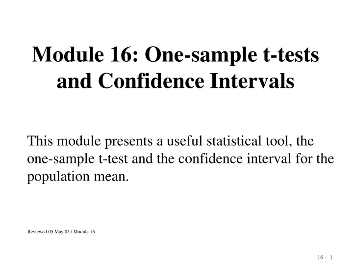
Module 16: One-sample t-tests and Confidence Intervals. This module presents a useful statistical tool, the one-sample t-test and the confidence interval for the population mean. Reviewed 05 May 05 / Module 16. The t-test and t Distribution.

E N D
Module 16: One-sample t-tests and Confidence Intervals This module presents a useful statistical tool, the one-sample t-test and the confidence interval for the population mean. Reviewed 05 May 05 / Module 16
The t-test and t Distribution What happens when we don't know the true value for the population standard deviation ? Suppose we have only the information from a random sample, n = 5, from the population of body weights, with = 153.0 lbs, and s = 12.9 lbs. When we had a value for the population parameter , we used the following formula:
t-test and t distribution (contd.) We do have an estimate of the population standard deviation, , namely the sample standard deviation s = 12.9 lbs. Hence, it seems reasonable to think that we should be able to use this estimate in some way. It is also reasonable to think that, if we substitute s for , we are substituting a guess at the truth for the truth itself and we will probably have to pay a price for doing so. So, what is the price? The essence of the situation is that, when we substitute a guess for the truth, we add noise to the system. The question then becomes one of characterizing this noise and taking it into account. Noise in this situation is equivalent to variability, so we are adding variability to the system. How much and exactly where?
t-test and t distribution (contd.) If we use this estimate, then we must make appropriate adjustments to the formula to account for the variability of this estimate. To properly account for this situation, we need to use a distribution different from the normal distribution. The appropriate distribution is the t distribution, which is very similar to the normal distribution for large sample sizes, but differs importantly for smaller samples, especially those with n < 30.
Confidence Interval for µ using s The appropriate formula, when = 0.05, is where t0.975(n-1) references the t distribution with n-1 degrees of freedom (df), specifically the point on that distribution below which lies 0.975 of the total area. For this situation, the correct number of degrees of freedom is one less that the sample size, i.e. df = n -1.
Tables for the t Distribution To obtain the values for the t distribution, see Table Module 2: The t distribution.
For the above situation, with n = 5, and s = 12.9 lbs, we have t0.975 (n-1) = t0.975 (4) = 2.776 so that the interval becomes: Example Given this confidence interval, would you believe that the population mean for the population from which this sample was selected had the value = 170.0 lbs?
Sample 95% Confidence Intervals for samples n = 5
Sample 95% Confidence Intervals for samples n = 20
Sample 95% Confidence Intervals for samples n = 50
Hypothesis Testing: = 153.0 lbs, s = 12.9 lbs • A random sample of n = 5 measurements of weights from a population provides a sample mean of = 153.0 lbs and a sample standard deviation of s = 12.9 lbs. Is it likely that the population mean has the value = 170 lbs.? • The hypothesis: H0: = 170 versus H1: ≠ 170 • The assumptions: Random sample from a normal distribution • The α- level:α = 0.05
The test statistic: • 5. The critical region:Reject H0: µ = 170 if the value calculated for t is not between ± t0.975(4) = 2.776 • 6. The result: • The conclusion: Reject H0: µ = 170 since the value calculated for t is not between ± 2.776.
This test was performed under the assumption that µ=170. Our conclusion is that our sample mean = 153.0 is so far away from µ=170 that we find it hard to believe that µ =170. That is, our observed value for the sample mean of = 153.0 is too rare for us to believe that = 170. Question: How rare is = 153.0 under the assumption that µ = 170?