Download

1 / 32
320 likes | 360 Views
Learn how hypothesis tests are used to investigate assumptions in data analysis, and how to interpret results using examples in a cattle study on hormone concentrations.

E N D
Hypothesis tests Statistical tests are used to investigate if the observed data contradict or support specific assumptions. In short, a statistical test evaluates how likely the observed data is if the assumptions under investigation are true. If the data is very unlikely to occur given the assumptions, then we do not believe in the assumptions. Hypothesis testing forms the core of statistical inference, together with parameter estimation and confidence intervals, and involves important new concepts like null hypotheses, test statistics, and p-values.
Example: Hormone concentration study As part of a larger cattle study, the effect of a particular type of feed on the concentration of a certain hormone was investigated. Nine cows were given the feed for a period, and the hormone concentration was measured initially and at the end of the period. The purpose of the experiment was to examine if the feed changes the hormone concentration. We obtain the sample mean 13.778 and the sample standard deviation 15.238. Thus, the difference is positive for eight of the nine cows. But is it strong enough for us to conclude that the feed affects the concentration?
Example: Hormone concentration study We consider the differences, denoted by d1,…,d9, during the period and assume that they are independent. Then μ is the expected change in hormone concentration for a random cow, or the average change in the population, and μ = 0 corresponds to no effect of the feed on the hormone concentration. The mean of the nine differences is 13.78, and we would like to know if this reflects a real effect or if it might be due to chance. Here we are interested in the null hypothesis corresponding to no difference between start and end measurements in the population.
Example: Hormone concentration study Now, the average difference 13.78 is our best “guess” for μ, so it seems reasonable to believe in the null hypothesis if it is “close to zero” and not believe in the null hypothesis if it is “far away from zero”. So we might ask: If μ is really zero (if the hypothesis is true), then how likely is it to get an estimatethat is as far or even further away from zero than the 13.78 that we actually got? A t-test can answer that question. Let The numerator is just the difference between the estimate of μ and the value of μ if the hypothesis is true. We then divide it by the standard error.
Example: Hormone concentration study If μ = 0 (the hypothesis is true), then Tobs is an observation from the t8 distribution (the number of degrees of freedom is n−1, here 9 − 1 = 8). In particular, we can compute the probability of getting a T-value which is at least as extreme as 2.71 by Here T is a t8 distributed variable and the second equality follows from the symmetry of the t distribution. This probability is called the p-value. If the p-value is small then the observed value Tobs is extreme, so we do not believe in the null hypothesis and reject it. If, on the other hand, the p-value is large then the observed value Tobs is quite likely, so we cannot reject the hypothesis. In this case the p-value is only 2.6%, so the T-value of 2.71 is quite unlikely if the true value of μ is zero. Hence, we reject the null hypothesis.
Example: Hormone concentration study Usually we use a significance level of 5%; that is, we reject the hypothesis if the p-value is ≤ 0.05 and fail to reject it otherwise. This means that the null hypothesis is rejected if |Tobs| is larger than or equal to the 97.5% quantile of the tn−1 distribution, which is in this Case 2.31. Hence, an observed T-value outside (−2.31, 2.31) leads to rejection of the null hypothesis.
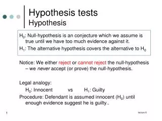
Concepts of hypothesis test • Null hypothesis. A null hypothesis is a simplification of the statistical model and is as such always related to the statistical model. Hence, no null hypothesis exists without a corresponding statistical model. A null hypothesis typically describes the situation of “no effect” or “no relationship”, such that rejection of the null hypothesis corresponds to evidence of an effect or relationship. • Alternative hypothesis. There is a corresponding alternative hypothesis to every null hypothesis. The alternative hypothesis describes what is true if the null hypothesis is false. Usually the alternative hypothesis is simply the complement of the null hypothesis.
Concepts of hypothesis test • Test statistic. A test statistic is a function of the data that measures the discrepancy between the data and the null hypothesis—with certain values contradicting the hypothesis and others supporting it. Values contradicting the hypothesis are called critical or extreme. • p-value. The test statistic is translated to a p-value—the probability of observing data which fit as bad or even worse with the null hypothesis than the observed data if the hypothesis is true. A small p-value indicates that the observed data are unusual if the null hypothesis is true, hence that the hypothesis is false.
Concepts of hypothesis test • Rejection. The hypothesis is rejected if the p-value is small; namely, below (or equal to) the significance level, which is often taken to be 0.05. With statistics we can at best reject the null hypothesis with strong certainty, but we can never confirm the hypothesis. If we fail to reject the null hypothesis, then the only valid conclusion is that the data do not contradict the null hypothesis. A large p-value shows that the data are in fine accordance with the null hypothesis, but not that it is true. • Quantification of effects. Having established a significant effect by a hypothesis test, it is of great importance to quantify the effect. For example, how much larger is the expected hormone concentration after a period of treatment? Moreover, what is the precision of the estimates in terms of standard errors and/or confidence intervals?
Concepts of hypothesis test In many cases, the interest is in identifying certain effects. This situation corresponds to the alternative hypothesis, whereas the null hypothesis corresponds to the situation of “no effect” or “no association.” This may all seem a little counterintuitive, but the machinery works like this: with a statistical test we reject a hypothesis if the data and the hypothesis are in contradiction; that is, if the model under the null hypothesis fits poorly to the data. Hence, if we reject the null hypothesis then we believe in the alternative, which states that there is an effect. In principle we never accept the null hypothesis. If we fail to reject the null hypothesis we say that the data does not provide evidence against it. This is not a proof that the null hypothesis is true, but it only indicates that the model under the alternative hypothesis does not describe the data (significantly) better than the one under the null hypothesis.
t-tests Consider the hypothesis for a fixed value θ0. Data for which the estimate for θj is close to θ0 support the hypothesis, whereas data for which the estimate is far from θ0 contradict the hypothesis; so it seems reasonable to consider the deviation. can be used as a test statistic. An extreme value of Tobs is an indication that the data are unusual under the null hypothesis, and the p-value measures how extreme Tobs is compared to the tn−p distribution.
t-tests If the alternative is two-sided, HA:θj≠ θ0, then values of Tobs that are far from zero—both small and large values—are critical. Therefore, the p-value is where T~ tn−p. If the alternative is one-sided, HA:θj > θ0, then large values of Tobs are critical, whereas negative values of Tobs are considered in favor of the hypothesis rather than as evidence against it. Hence the p-value is P(T ≥ Tobs). Similarly, if the alternative is one-sided, HA:θj < θ0, then only small values of Tobs are critical, so the p-value is P(T ≤ Tobs). The significance level is usually denoted α, and it should be selected before the analysis. Tests are often carried out on the 5% level corresponding to α = 0.05, but α = 0.01 and α = 0.10 are not unusual.
t-tests For a hypothesis with a two-sided alternative, the hypothesis is thus rejected on the 5% significance level if Tobs is numerically larger than or equal to the 97.5% quantile in the tn−p distribution; that is, if |Tobs| ≥ t0.975,n−p. Similarly, with a one-sided alternative, HA:θj > θ0, the hypothesis is rejected if Tobs ≥ t0.95,n−p. Otherwise, we fail to reject the hypothesis, and the model under the alternative hypothesis does not describe the data significantly better than the model under the null hypothesis. In order to evaluate if the null hypothesis should be rejected or not, it is thus enough to compare Tobs or |Tobs| to a certain t quantile. But we recommend that the p-value is always reported.
Type I and type II errors Four scenarios are possible as we carry out a hypothesis test: the null hypothesis is either true or false, and it is either rejected or not rejected. The conclusion is correct whenever we reject a false hypothesis or do not reject a true hypothesis. Rejection of a true hypothesis is called a type I error, whereas a type II error refers to not rejecting a false hypothesis; see the chart below. We use a 5% significance level α. Then we reject the hypothesis if p-value ≤ 0.05. This means that if the hypothesis is true, then we will reject it with a probability of 5%. In other words: The probability of committing a type I error is the significance level α.
Type I and type II errors The situation is analogous to the situation of a medical test: Assume for example that the concentration of some substance in the blood is measured in order to detect cancer. (Thus, the claim is that the patient has cancer, and the null hypothesis is that he or she is cancer-free.) If the concentration is larger than a certain threshold, then the “alarm goes off” and the patient is sent for further investigation. (That is, to reject the null hypothesis, and conclude that the patient has cancer.) But how large should the threshold be? If it is large, then some patients will not be classified as sick (failed to reject the null hypothesis) although they are sick due to cancer (type II error). On the other hand, if the threshold is low, then patients will be classified as sick (reject the null hypothesis) although they are not (type I error).
Type I and type II errors • For a general significance level α, the probability of committing a type I error is α. Hence, by adjusting the significance level we can change the probability β of rejecting a true hypothesis. This is not for free, however. If we decrease α we make it harder to reject a hypothesis—hence we will accept more false hypotheses, so the rate of type II errors will increase. • The probability that a false hypothesis is rejected is called the power of the test, and it is given by (1−β). We would like the test to have large power (1−β) and at the same time a small significance level α, but these two goals contradict each other so there is a trade-off. As mentioned already, α = 0.05 is the typical choice. Sometimes, however, the scientist wants to “make sure” that false hypotheses are really detected; then α can be increased to 0.10, say. On the other hand, it is sometimes more important to “make sure” that rejection expresses real effects; then α can be decreased to 0.01, say.
Example: Parasite counts for salmons The salmon data with two samples corresponding to two different salmon stocks, Ätran or Conon, are obtained. If αÄtran = αConon then there is no difference between the stocks when it comes to parasites during infections. Hence, the hypothesis is H0: αÄtran = αConon. If we define θ = αÄtran−αConon then the hypothesis can be written as H0:θ = 0. The t-test statistic is therefore
Example: Parasite counts for salmons The corresponding p-value is calculated as Hence, if there is no difference between the two salmon stocks then the observed value 4.14 of Tobs is very unlikely. We firmly reject the hypothesis and conclude that Ätran salmons are more susceptible to parasites than Conon salmons.
t-tests and confidence intervals H0:θj = θ0 is rejected on significance level α against the alternative HA:θj≠θ0 if and only if θ0 is not included in the 1−α confidence interval. This relationship explains the formulation about confidence intervals; namely, that a confidence interval includes the values that are in accordance with the data. This now has a precise meaning in terms of hypothesis tests. If the only aim of the analysis is to conclude whether a hypothesis should be rejected or not at a certain level α, then we get that information from either the t-test or the confidence interval. On the other hand, they provide extra information on slightly different matters. The t-test provides a p-value explaining how extreme the observed data are if the hypothesis is true, whereas the confidence interval gives us the values of θ that are in agreement with the data.
Example: Stearic acid and digestibility Recall the linear regression model for the digestibility data where e1,…,en are residuals. The hypothesis that there is no relationship between the level of stearic acid and digestibility is tested by the test statistic where the estimate −0.9337 and its standard error 0.0926 are obtained from the data. The value of Tobs should be compared to the t7 distribution.
Example: Stearic acid and digestibility For the alternative hypothesis HA:β≠ 0 we get and we conclude that there is strong evidence of an association between digestibility and the stearic acid level—the slope is significantly different from zero. Since the estimate −0.9337 of slope is negative, we conclude that the digestibility percentage decreases as the percentage of stearic acid increases.
ANOVA (analysis of variance) • In the one-way ANOVA setup with k groups, the group means α1,…,αk are parameters, and we write the one-way ANOVA model • where g(i) = xi is the group that corresponds to yi. The remainder terms e1,…,en are independent and N(0,σ2) distributed. In other words, it is assumed that there is a normal distribution for each group, with means that are different from group to group and given by the α's but with the same standard deviation in all groups (namely, σ) representing the within-group variation. The parameters of the model are α1,…,αk and σ, where αj is the expected value (or the population average) in the jth group. In particular, we are often interested in the group differences αj−αl, since they provide the relevant information if we want to compare the jth and the lth group.
Standard error in one-way ANOVA • Consider the one-way ANOVA model • where g(i) denotes the group corresponding to the ith observation and e1,…,en are independent and N(0,σ2) distributed. Then the estimate for the group means α1,…,αk are simply the group averages, and the corresponding standard errors are given by • It suggests that mean parameters for groups with many observations (large nj) are estimated with greater precision than mean parameters with few observations.
Standard error in one-way ANOVA • In the ANOVA setup the residual variance s2 is given by • which we call the pooled variance estimate. In the one-way ANOVA case we are very often interested in the differences or contrasts between group levels rather than the levels themselves. Hence, we are interested in quantities αj−αl for two groups j and l. Then the estimate is simply the difference between the two estimates, and the corresponding standard error is given by • The formulas above are particularly useful for two samples (k = 2).
Example: Dung decomposition • An experiment with dung from heifers was carried out in order to explore the influence of antibiotics on the decomposition of dung organic material. As part of the experiment, 36 heifers were divided into six groups. All heifers were fed a standard feed, and antibiotics of different types (alpha-Cypermethrin, Enrofloxacin, Fenbendazole, Ivermectin, Spiramycin) were added to the feed for heifers in five of the groups. No antibiotics were added for heifers in the remaining group (the control group). For each heifer, a bag of dung was dug into the soil, and after eight weeks the amount of organic material was measured for each bag.
Null hypothesis for ANOVA • Consider the comparison of groups • where g(i) is the group that observation i belongs to and e1,…,en are residuals. As usual, k denotes the number of groups. In a typical linear model, it tests the null hypothesis that αi = 0. However, in this study we are interested in whether there is no difference between the groups. Thus, the null hypothesis is given by • and the alternative is the opposite; namely, that at least two α's are different.
F-tests in ANOVA • Since only large values of F are critical, we have • where F follows the F(k−1,n−k) distribution. The hypothesis is rejected if the p-value is 0.05 or smaller (if 0.05 is the significance level). In particular, H0 is rejected on the 5% significance level if Fobs ≥ F0.95,k−1,n−k.
F-test • If the null hypothesis is true, then Fobs comes from a so-called F distribution with (k−1,n−k) degrees of freedom. Notice that there is a pair of degrees of freedom (not just a single value) and that the relevant degrees of freedom are the same as those used for computation of MSgrp and MSe. The density for the F distribution is shown for three different pairs of degrees of freedom in the left panel below.
F-test • If there is no difference between any of the groups (H0 is true), then the group averages will be of similar size and be similar to the total mean . Hence, MSgrp will be “small”. On the other hand, if groups 1 and 2, say, are different (H0 is false), then the group means will be somewhat different and cannot be similar to —hence, MSgrp will be “large”. “Small” and “large” should be measured relative to the within-group variation, and MSgrp is thus standardized with MSe. We use • as the test statistic and note that large values of Fobs are critical; that is, not in agreement with the hypothesis.
Example: Antibiotics on decomposition • The values are listed in an ANOVA table as follows: • The F value 7.97 is very extreme, corresponding to the very small p-value. Thus, we reject the hypothesis and conclude that there is strong evidence of group differences. Subsequently, we need to quantify the conclusion further. Which groups are different and how large are the differences?