Download
1 / 77
770 likes | 781 Views
Robert W. Grubbström FVR RI, FLO K. Linköping Institute of Technology, Sweden Mediterranean Institute for Advanced Studies, Š empeter pri Gorici, Slovenia. robert@grubbstrom.com. Work-in-Progress, Capital Costs and Tradeoffs.

E N D
Robert W. Grubbström FVR RI, FLO K Linköping Institute of Technology, Sweden Mediterranean Institute for Advanced Studies, Šempeter pri Gorici, Slovenia robert@grubbstrom.com Work-in-Progress, Capital Costs and Tradeoffs Keynote Address, XVI SUMMER SCHOOL "FRANCESCO TURCO" Abano, September 14-16, 2011
To Alessandro and all Italian Colleagues and Friends: Thank you very much for inviting me and my wife Anne-Marie to theXVI SUMMER SCHOOL "FRANCESCO TURCO"
The Italian Marquis and engineer Vilfredo Pareto, 1848-1923, was born i Paris. He wrote a thesis in solid mechanics with the title Principes fondamentaux de l’équilibre de corps solides, which he defended at the Technical University of Turin in 1869. He was appointed ”ordinary” Professor of economie politique at the University of Lausanne in 1894. He created ”Pareto’s law”, which later has become known as the ”80/20-rule”. He contributed to the foundation of welfare economics, by defining optimality in an economic system as a state from which no one can become better off without somebody else becoming worse off (Pareto Optimality).
The First Industrial Engineer Vilfredo Pareto, 1848-1923
Abstract Production is the transformation from one set of resources into a second set of – hopefully - more valuable resources. This transformation takes time and creates a need for capital with consequential capital costs, since resources are utilised before resulting products are in place. In the meantime resources are earmarked as work-in-progress. This keynote lecture discusses the methodology for determining capital costs from a financial point of view enabling the capital costs of work-in-progress to be evaluated in a compatible way as any other capital costs pertaining to investments in general. The main emphasis is laid on the thesis that payments are the ultimate consequences of economic activities. Therefore for determining the true capital costs, monetary payments should be traced and measured as closely as possible as to their amount, timing and risk. Topics to be included are tradeoffs between work-in-progress and capital costs, and methodology for determining capital costs for production with complex structures including recycling activities, dynamic lotsizing, inter alia. The traditional Average Cost (AC) method is contrasted with the Net Present Value (NPV) principle and its related Annuity Stream measure.
Today’s Agenda • Brief on financial methodology • Application to EOQ/EPQ problem types • Dynamic lotsizing • MRP systems • Recycling • Balancing Queueing and Capacity Costs • Conclusions
(i) Arguments for emphasising monetary streams(rather than cost assumptions) • The ultimate economic consequences of all activities in a company are in the form of monetary streams. This is the closest one can come to measuring the real economic performance of the firm. • This is emphasised in particular, when a company is created, and when it is on the verge of collapsing. • Modern legislation stresses the need to keep track of monetary consequences, for instance by requiring a statement of changes in financial position. • Overwhelming theory requires that cash flows should be evaluated by their resulting Net Present Value (NPV), or by some equivalent measure such as their corresponding Annuity Stream.
(i) Arguments for using continuous time(rather than discrete time) • A discrete time scale is embedded in a continuous time scale, so continuous time is more general. • Globalisation makes time more continuous than before from a practical point of view. • Often it is easier to solve problems with continuous variables. • In discrete problems, there might be periods with no events, but empty periods do not exist in continuous time.
Initial Capital Continuous Discrete time Capital accumulation in discrete and continuous time
Continuous interest rate Length of discrete period Discrete interest rate So we can turn any discrete time problem into a continuous time problem using the corresponding continuous interest rate ρ.
The Net Present Value may therefore be written in a completely general form:
where T is the relevant time period The corresponding Annuity Stream is the constant flow of payments during a given timeperiod T giving rise to a given NPV:
Example of the use of the Annuity Stream Compare the purchase of either of two similar machines. Which to choose? A or B? NPV of costs: NPVA and NPVB Economic life: TA and TBChoose the one with the lowest of:
Risk and Interest A simplest model to include risk is by adding anincrement to the interest rate. Consider a project with the stake –G and risk (probability) q of loosing any outcome per time period with the expected outcome S, if every period is successful:
The interest increment r compensating risk q is therefore The project is successful with the probability (1-q)-N yielding the outcome S. Assume that the project outcome grows with time according to S = G(1+r)N. The expected NPV then becomes So if Risk and Interest II This is a simple interpretation of the tradeoff between risk (security) and interest for a risk-neutral person.
Hadley, G., A comparison of order quantities computed using the annual cost and the discounted cost, Management Science, 10(3), 1964, 472-476.
Grubbström, R.W., A principle for determining the correct capital costs of inventory and work-in-progress, IJPR, 18(2), 1980, 259-271.
Inventory pattern Payment streams Q Q Q Q Average=Q/2 time Q/D pD time -K-cQ -K-cQ -K-cQ -K-cQ Average Cost versus Annuity Stream
Payment streams Inventory pattern Q Q Q Q Average=Q/2 time Q/Daver pQ pQ pQ pQ time -cDaver -K -K -K -K Demand in batches Q, production rate=average demand rate
Inventory pattern Payment streams time Q/D pD time cq cq cq cq -K -K -K -K Inbetween EPQ pattern, production rate=q, average demand rate=D
Brian G. Kingsman, 1939-2003 EOQ when future price changes: Grubbström, R.W., Kingsman, B.G., Ordering and Inventory Policies for Step Changes in the Unit Item Cost: A Discounted Cash Flow Approach, Management Science, 50(2), 2004, 253–267.
Optimal inventory pattern Stationary sequence atnew price time T Equation governingsequence of intervals Example: Assume a price increase at T: Then the optimal solution will be a sequence of increasing or decreasing order quantities followed by a larger quantity immediately prior to T.
Background William Stanley Jevons 1835-1882 The Newsboy (Newsvendor) problem is probably the simplest of all stochastic inventory problems, involving a one-time purchase decision and a stochastic sales outcome. As an investment, it can be interpreted as the simplest stochastic version of the point-in, point-out investment problem of William Stanley Jevons (1871).
Bertrand Russel: Forethought – Which involves doing unpleasant things now for the sake of pleasant things in the future, is one of the most important marks of the development of man. Bertrand Russel 1872-1970
To choose the optimal time for the asset to mature, which is to choose T that maximises RewardR(T) Time of investment T Necessary optimisation condition Outlay-G Jevons’ Problem
A Newsboy problem with Compound Renewal Demand One of simplest business problems is when you bring a bundle of products to the market place, but you don’t know how much to bring. If too much, then you’ll have a loss from discarding the leftovers, and if to few, you will loose customers to someone else. This is the classical Newsboy problem. But life can be much more complicated. Your customers may come at intervals to your outlet, and they each require different amounts. Here, there are two uncertainties, one concerning the timing, and one concerning the amounts. However, this second much more involved situation can be modelled in exactly the same way as the first simple case, if the probability distribution is designed in a special way and you want to maximise your Net Present Value.
time -cQ Newsboy with Compound Renewal Demand II First customer arrives buying D1items Second customer arrives buying D2items Third customer arrives buying D3items Fourth customer arrives buying D4items Buy/make/purchase Q items time
Grubbström, R.W., The Newsboy problem when customer demand is a compound renewal process, EJOR, 203(1), 2010, 134-142.
Time reference point for discounting Very recent article suggesting an explanation to differences in Average Cost Approach and Annuity Stream Principle forEOQ/EPQ models Beullens, P., Janssens, G.K., Holding Costs under Push or Pull Conditions - The Impact of the Anchor Point, EJOR, 215(1), 2011, 895-908.
Dynamic Lotsizing
Background • Single product • No backlogging allowed • Finite horizon • Given requirements di at given times ti The Wagner-Whitin(optimal, 1958) and theSilver-Meal(heuristic, 1973) algorithms for dynamic lotsizing are normally presented in terms of an average cost function in discrete time. An additional forward optimal dynamic lotsizing algorithm has been presented recently called theTriple Algorithm. This new algorithm may be applied either time is discreteorcontinuous, and either the traditional average costor the Net Present Value (Annuity Stream) is the objective function.
Problem To choose the amount to produce (or not to produce) at each time satisfying given requirements and optimising an objective function (NPV or AC)
Obvious observations (i) When the setup cost K is very high compared to the holding cost h, there can only be one setup at the very beginning of the process (the All-At-Once, @1, solution). (ii) With a very low setup cost K, there must be a setup at every time a non-zero requirement occurs (the Lot-For-Lot, L4L, solution). Therefore, the domain in which dynamic lotsizing exists as a non-trivial problem, is when this ratio is neither high, nor low.
Cannot be optimal! requirements production production inner corner contact Inner Corner Property (necessary for optimality) The Inner-Corner Condition is valid for either DiscreteorContinuous Time problems and either the Average Cost Approach or the NPV/Annuity Stream Principle is used. Furthermore, this condition applies also toany Multi-Product Assembly System with arbitrarily complex Product Structures. This turns the Dynamic Lotsizing Problem into a zero/one problem: To Produce or Not to Produce time
Grubbström, R. W., Bogataj, M., Bogataj, L., Optimal Lotsizing within MRP Theory, Annual Reviews in Control, 34(1), 2010, 89–100.
Cumulative Production Cumulative Requirements Inner Corner Conditions 2n-1 alternatives time Staircase Functions
Values of function 2n-1 n 2n-1 1 1 2 2 3 4 4 8 5 16 10 512 15 16 384 20 524 288 n 2n-1 25 16 777 216 30 536 870 912 35 17 179 869 184 40 549 755 813 888 45 17 592 186 044 416 50 562 949 953 421 312 100 633 825 300 114 115·1015
Complexity issues for general assembly systems are studied in: Grubbström, R. W., Tang, O., The space of solution alternatives in the optimal lotsizing problem for general assembly systems applying MRP theory, IJPE, Article in Press, 2010, doi:10.1016/j.ijpe.2011.01.012.
According to the Silver-Meal algorithm the time average of a setup cost and holding costs is computed starting at the time of each replenishment and proceeding in steps of one time unit. As soon as there is an increase in this average cost measure, it is time for a new replenishment. In our terminology, we interpret the average cost expression as the annuity of the out-payments. Therefore, A(k) is computed for k = 2, 3, … . When A(k+1) > A(k), the order at is determined as . Silver-Meal Algorithm
Thomson M. Whitin, b. 1923 Edward A. Silver, b. 1937
Thomson M. Whitin, b. 1923 Harvey M. Wagnerb. 1931 Thomson M. Whitinb. 1923
NPV where Bellman Equation for Wagner-Whitin Algorithm in continuous time:
Max Area requirements j Triple Algorithm: Basic Principle If Max Area < K/h, then no setup within interval. If Max Area >K/h, then at least one setup within interval. time k i
What the Triple Algorithm does 1. The algorithm discards setups which are too far apart by determining the latest next setup. 2. The algorithm discards setups which are too close by determining the earliest next setup. 3. When determining the local optimum for each pair of boundaries, the algorithm discards (several) non-optimal, but feasible intermediate setups, thus limiting the number of remaining paths. 4. By checking triples generated at adjacent stages, the algorithm discards incompatible triples, also limiting the set of feasible paths.
2(30-1)=536 870 912 Optimum or 1, 4, 7, 9, 13, 20, 26, 31 1 , 6 , 9, 13, 20, 26, 31 Example of Triple Algorithm Time Demand 0 30 1.06862366199493 70 1.54904127120972 50 8.83765518665314 60 11.3184928894043 40 20.7954579591751 70 30.6325888633728 40 35.2663880586624 60 42.0667839050293 60 44.3357878923416 50 44.5454096794128 20 49.7288924455643 10 56.2518310546875 70 59.0022355318069 60 60.3511023521423 60 67.0475560426712 30 68.5251235961914 30 77.9082041978836 10 87.3202967643738 20 91.9080477952957 80 92.3076820373535 10 93.0928784608841 80 95.0556540489197 20 101.98431789875 50 103.182997107506 20 112.785895466805 90 117.854326367378 90 118.950929045677 30 120.846487879753 70 123.841343522072 30 1 1 4 7 * 1 6 8 * 1 6 9 4 6 8 * 4 7 9 * 4 7 10 * 6 9 13 * 6 9 14 7 9 13 * 7 9 14 * 9 13 19 * 9 13 20 9 13 19 * 9 13 20 * 13 20 24 * 13 20 25 * 13 20 26 13 20 24 * 13 20 25 * 13 20 26 * 20 26 31 20 26 31 1 1 4 7 * 1 6 9 4 7 9 * 6 9 13 7 9 13 * 9 13 20 9 13 20 * 13 20 26 13 20 26 * 20 26 31 20 26 31 1 1 4 7 * 1 6 8 * 1 6 9 4 6 8 * 4 7 9 * 4 7 10 * 6 9 13 * 6 9 14 7 9 13 * 7 9 14 * 9 13 19 * 9 13 20 9 13 19 * 9 13 20 * 13 20 24 * 13 20 25 * 13 20 26 13 20 24 * 13 20 25 * 13 20 26 * 20 26 31 20 26 31
MRP Systems