Download
1 / 35
350 likes | 453 Views
Why, Where and How to Use the - Model Josef Widder Embedded Computing Systems Group widder@ecs.tuwien.ac.at INRIA Rocquencourt, March 10, 2004. Work in Progress. Motivation Ideas Our Approach First Results in certain types of networks. Overview.

E N D
Why, Where and How toUse the - ModelJosef WidderEmbedded Computing Systems Groupwidder@ecs.tuwien.ac.atINRIA Rocquencourt, March 10, 2004
Work in Progress • Motivation • Ideas • Our Approach • First Results in certain types of networks
Overview • Why: Because classic results are straight forward but have drawbacks • Where: A glance at synchrony in real networks • How: Transfer of algorithm to real systems
Consensus • Dwork, Lynch, Stockmeyer 88 • Chandra, Toueg 96 • There exist algorithmic solutions if holds • is the upper bound on end-to-end message delays • What remains: Show that your system ensures
Diverse assumptions on • is known/unknown • hold always/from some time one/sufficiently long • holds for all/some (FD) msgs … [DLS88] / [CT96] • holds eventually somewhere … [ADFT03] These are weak assumptions, still is in there
Upper bounds do not look like this • Let’s assume = 8s and test it for a week • Approaches like [MF02] • delay of a protocol is 5 • delay should be at most 5s • let’s define = 1s
Can upper bounds be derived properly ? • Guarantees are (NP) hard to derive (scheduling, queuing) • problem must be simplified • simplification leads to incomplete guarantees
What do I have to analyze to ensure • local delays sender (processor load, task preemption, blocking factors) • outbound queues • net contention • inbound queues • local delays receiver (processor load, task preemption, blocking factors) This is hard, yet only delivers at some probability.
Assumption Coverage The probability that our assumptions hold during operation Our Starting Point: We can improve coverage by means of system models
The Model (t) ... Upper envelope of message delays at time t (t) ... Lower envelope of message delays at time t Since (t) is unbounded, local HW timers cannot timeout messages time(r) free algorithms
Described Behavior (rough sketch) end-to-end delays t
Coverage of C < 1 C = 1
Coverage of the - Model How large is states( ) ? And why is this interesting anyway ?
Consensus in Real Networks From FLP follows: Any solution to Consensus on a real network is a probabilistic solution … not even talking about coverage of fault models
How large is coverage improvement ? • Coverage cannot be worse than in assumption • if relation of and exists, improvement is large. • But even in networks without relation of and (if such exist?) • If by chance there exists just one case where holds while does not, coverage is improved
Performance termination times often look like hence: How large is ? • Step 1 timing uncertainty of networks • Step 2 establish , , and on given networks, for a given system model for given algorithms
Benchmark for Timing Uncertainty in clock synchronization the best precision one can reach is = - [LL84] … (1-1/n) comparison of two approaches in Ethernet • clock sync • their results • conclude where to use our model
Clock Sync in Ethernets • NTP [Mills] • Accuracy of ~1ms • SynUTC [http://www.auto.tuwien.ac.at/Projects/SynUTC/papers.html] • Accuracy of ~100ns Why is there a difference of 4 orders of magnitude?
Wherefrom comes the difference ? • NTP runs at application level • SynUTC runs low level • current clock value is directly copied onto the bus • upon message receipt, receiver’s clock value is written in the received message as well • interval based clock sync algorithms [SS03]
Conclusions from this comparison • low level clock sync • high level applications use tightly synchronized clocks • But how does this help us in solving Consensus? • Fast Failure Detector Approach [HLL02] ([CT96]: just FD messages must satisfy timing assumptions)
Fast Failure Detectors • low level failure detection • high priority FD messages … n = 16…1024
Performance (after Step 1) • Timing uncertainty differs in same network depending on the layer the algorithm runs in • should be reasonable good in lower levels • Step 2: establish , , and on given networks, for a given system model running given algorithms
Algorithms in Networks • Leader Election • Token Circulation (1x) • 1. 2. end-to-end delays ,
Theoretical Analysis • Leader Election • bc(leader) = ... wc(leader) = • one Token Circulation • bc(token) = 3 ... wc(token) = 3 • Leader Token • bc(comb) = 4 ... wc(comb) = 4
Establish Time Bounds • end-to-end delays • from decision to send a message until receivermakes its decision • = ts + trans + tr • = 2ts + trans + 2tr … message arrival laws rate of transmission to one p
Termination Times Leader Election Token Circulation
... by adding ... by examination Termination Times (2) Leader Election Token Round
Conclusions of Step 2a • during operation , do not only depend on the system • algorithms must be accounted as well • how many messages are sent network load • this was a toy example BUT
Deterministic Ethernet … CSMA/DCR • bus only one message on the medium at a time • deterministic collision resolution • upper bound on physical message transmission (i.e. trans not the end-to-end delay) • if a station wants to send a message at t1 and sends it at t2 (collision) then every station can at most send one message between t1 and t2
= - … is only relevant for one broadcast in fact the time difference for receiving n - f msgs Hot: First Results in Deterministic Ethernet
in deterministic Ethernet: but we require f+1 msgs: First Results (2) ... how many messages transferred during any message is in transit
First Results in Deterministic Ethernet (3) • n = 1024 and f = 511 … crash faults, hence n > 2f • derive properties which are equivalent to 2 in the system model • results apply in TDMA networks as well (due to inefficiency of the bus arbitration might be even smaller)
Conclusions • - Model reaches higher assumption coverage • small timing uncertainty in lower network levels • , , , and are related to • real network • algorithm • remains within reasonable bounds