Download
1 / 15
150 likes | 156 Views
Routing in WSNs through analogies with electrostatics. December 2005 L. Tzevelekas I. Stavrakakis. Recent developments in routing for WSNs. Papers on this topic:

E N D
Routing in WSNs through analogies with electrostatics December 2005 L. Tzevelekas I. Stavrakakis
Recent developments in routing for WSNs • Papers on this topic: • M. Kalantari and M. Shayman, “Routing in wireless ad hoc networks by analogy to electrostatic theory,” in Proc. IEEE ICC, Paris, France, June 2004. • M. Kalantari and M. Shayman, “Energy efficient routing in wireless sensor networks,” in Proc. Conference on Information Sciences and Systems, Princeton University, NJ, Mar. 2004. • N. T. Nguyen, A.-I A. Wang, P. Reiher, and G. Kuenning, “Electric-field based routing: A reliable framework for routing in MANETs,” ACM Mobile Computing and Communications Review, vol. 8, no. 1, pp. 35– 49, Apr. 2004. • S. Toumpis and L. Tassiulas, “Packetostatics: Deployment of Massively Dense Sensor Networks as an Electrostatics Problem,” Proc. INFOCOM 2005.
Back to the basics • Sensors are sources of information => positive charges in electromagnetism • Central node is the sink of information => negative charges in electromagnetism • Network is like a non-homogeneous dielectric media • Routing scheme based on changing the permittivity factor of media: high values in places with high residual energy, i.e. more traffic through that region low values for regions with low residual energy, i.e fewer traffic through that region
Mathematical formulation • N sensors on a plane region A • Sensors communicate through wireless multi-hop links to a central node entity called the sink • On happening of events, the nearest sensor chooses to report it to the sink • Sensors have limited amounts of residual energy (known at each time unit) • Events happening with a known spatial density rate: r(z) ≥ 0, z denotes a point (x,y) on the plane Rate of events inside α:
Mathematical formulation • Sensors are not mobile and their locations are known • For routing purposes in the network: • We keep a direction for every point z of the network • Sensor placed at point z uses direction defined at that point and forwards traffic to the closest sensors to this direction • Assume the direction to be a continuous function of z • Each sensor i is associated with a weight wi>0 denoting the average rate of messages generated by sensor i • Assign weight to the central node as follows: w0=
Mathematical formulation • Define a path as a directed curved line starting at sensor i and ending at the central node • Each sensor i is associated with a path pi (‘abstract’ paths, not constrained by locations of intermediate nodes) • The amount of load on that path is wi (same as the rate of messages generated at the starting node) • Define a vector field on A to be the load density vector fieldat point z, denoted by D(z):
Mathematical formulation • Based on the definition of D(z), one can prove that • C is a closed contour in the region A • dn is a differential vector normal to the contour at each point of its boundary • w is the algebraic sum of the weights of the nodes inside the closed contour • the above equation is analogous to Gauss’s law in the electrostatics theory
Mathematical formulation • Analytical explanation of the formula: the rate at which messages exit a contour is the algebraic sum of the weights of the nodes that are inside that contour (net amount of sources inside that contour) Defining the net amount of sources in the network as: one can express the equation in differential form as follows: where
Energy efficient routing • Define the concept of load flow lines • Similar to the electric flux lines • Family of 2-D curved lines • Always tangent to the direction of D(z) • Orientation same as orientation of D(z) • Cannot intersect except at a source or a destination • Start at sources and end at the destination • To find pi we start at the place of sensor i and follow the direction of the load flow lines
Energy efficient routing • To associate the paths with the residual energy at each sensor, we define the scalar field of the residual energy of the network as a function of z: • Make use of the fact that |D(z)| represents the communication activity at point z (= the energy dissipation at point z) • To achieve uniform energy dissipation overall in the region A we form the following quadratic minimization problem:
Energy efficient routing • Solving the previous minimization problem leads to the introduction of the potential function U it can be shown that the optimal solution for D*(z) satisfies and this is the necessary and sufficient condition for having a conservative vector field D*(z) Such a vector field can equivalently be described through the gradient of a scalar function called the potential function And the differential equations then become: (poisson equation)
Energy efficient routing • Finally taking into account the scalar field ω(z, t) of the residual energy, we obtain the following quadratic minimization problem where K(z) is a scalar weight function representing where in the network we prefer to have a higher load and where we want to have less communication activity in order to save the energy of the nodes
Results • sensors of the network are distributed in a 1000m x 1000m square • the number of sensors is N = 441 • the central node has been placed in the center of the network area • a Poisson process is responsible for generating events • distributed the initial energy of 20000 units among the sensors. • the initial energy of the sensors is inversely proportional to their distance from the central node. • the transmission range of each sensor is 85m
Results Numerical computation of the values of the potential function U Direction of D*(z) is calculated as the gradient of U Paths from sensors to the destination are found by following these segment lines
Results • Comparison of • the performance of routes found based on D (z) • the performance of routes found with the shortest path method • for several experiments