Download
1 / 19
190 likes | 320 Views
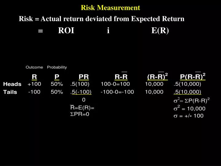
Risk Measurement. Risk = Actual return deviated from Expected Return = ROI i E(R). E(R) = S P i R i = R = Expected Return Ex-ante = Future Events Ex-post = Historical Data s = Standard Deviation = risk s 2 = Variance = S P(R-R) 2.

E N D
Risk Measurement • Risk = Actual return deviated from Expected Return • = ROI i E(R)
E(R) = SPiRi = R = Expected Return • Ex-ante = Future Events • Ex-post = Historical Data • s = Standard Deviation = risk • s2= Variance = SP(R-R)2
Standard Deviation, Sigma, Expected Return • -(2)s -(1)s R (1)s (2)s • - 100 0 +100
Returns on Alternative Investments • I. Discrete Probability Distribution • Estimated Rate of Return • State of the T- High U.S. Market 2-Stock • Economy Probability Bills Tech Collections Rubber Portfolio Portfolio • Recession 0.1 8.0% -22% 28.0% 10.0% -13.0% 3.0% • Below average 0.2 8.0 -2.0 14.7 -10.0 1.0 6.4 • Average 0.4 8.0 20.0 0.0 7.0 15.0 10.0 • Above average 0.2 8.0 35.0 -10.0 45.0 29.0 12.5 • Boom 0.1 8.0 50.0 -20.0 30.0 43.0 15.0 • Expected Ret (k) 8.0 17.4% 1.7% 13.8% 15.0% 9.6% • Std. Dev. (s) 0.0 20.0 13.4 18.8 15.3 3.3 • Coef. of Var. (CV) 0 1.1 7.9 1.4 1.0 0.3 • Risk (b) 0.0 1.29 -0.86 0.68 1.00
Returns on Alternative Investments • II. Continuous Probability Distribution • Probability of Occurrence • 0.4 • Market Portfolio • -45 -30 -15 0 15 30 45 60 75 • k Rate of Return (%)
Calculation of k • n • k = S Piki • i=1 • kHigh Tech = 0.10(-22.0%) + 0.20(-2.0%) • + 0.40(20.0%) + 0.20(35.0%) • + 0.10(50.0%) = 17.4% • kT-bills = 8.0% • kCollections = 1.7% • kU.S.Rubber = 13.8% • kM = 15.0%
Calculation of s • n • s = VARIANCE = s2 = S (ki - k)2Pi • i=1 • sHigh Tech = [(-22.0 - 17.4)2 0.10 + (-2.0 - 17.4)2 0.20 • + (20.0 - 17.4)2 0.40 + (35.0 - 17.4)2 0.20 • + (50.0 - 17.4)2 0.10]1/2 = (401.1)1/2 = 20.0% • sT-bills = 0.0% • sCollections = 13.4% • sU.S.Rubber = 18.8% • sM = 15.3%
Continuous Probability Distributions: High Tech, U.S. Rubber, & T-Bills • Probability of Occurrence • T-Bills • High Tech • U.S. Rubber • -45 -30 -15 0 8 15 30 45 60 • Rate of Return (%)
Calculation of CV • CV = s • k • CVT-bills = 0.0% / 8.0% = 0.0 • CVHighTech = 20.0% / 17.4% = 1.1 • CVCollections = 13.4% / 1.7% = 7.9 • CVU.S. Rubber = 18.8% / 13.8% = 1.4 • CVMarket = 15.3% / 15.0% = 1.0
Ranking of Investment Alternatives • Expected • Return Risk s CV • Security k s Ranking CV Ranking • High Tech 17.4% 20.0% 5 1.1 3 • Market 15.0 15.3 3 1.0 2 • U.S. Rubber 13.8 18.8 4 1.4 4 • T-bills 8.0 0.0 1 0.0 1 • Collections 1.7 13.4 2 7.9 5 • 1 = Least risky • 5 = Most risky
Portfolio Return & Standard Deviation • 2-Stock Portfolio Return: 50% High Tech and 50% Collections • kp = Sn wiki • i=1 • kp = 0.5(17.4%) + 0.5(1.7%) = 9.6% • Standard Deviation: • State of the Expected Return • Economy Prob. High Tech Collections 2-Stk Portfolio • Recession 0.10 -22.0% 28.0% 3.0% • Below average 0.20 -2.0 14.7 6.4 • Average 0.40 20.0 0.0 10.0 • Above average 0.20 35.0 -10.0 12.5 • Boom 0.10 50.0 -20.0 15.0
Portfolio Return & Standard Deviation • By considering the portfolio return in each state of the economy, we have another way of calculating kp: • kp = 0.10(3.0%) + 0.20(6.4%) + 0.40(10.0%) • + 0.20(12.5%) + 0.10(15.0%) = 9.6% • Given the distribution of returns for the portfolio, we can calculate the portfolio’s sp and CV: • sp = [(3.0 - 9.6)2 0.10 + (6.4 - 9.6)2 0.20 • + (10.0 - 9.6)2 0.40 + (12.5 - 9.6)2 0.20 • + (15.0 - 9.6)2 0.10]1/2 = 3.3% and • CVp = 3.3% / 9.6% = 0.34
Portfolio Returns & Risk: High Tech & Collectionsoptional question integrated case • Rate of Return (%) • 20 • 16 • 12 kP • 8 • 4 • 0 • 0 20 40 60 80 100 % in High Tech • Standard Deviation sP (%) • 20 • 16 • 12 sP • 8 • 4 • 0 • 0 20 40 60 80 100 % in High Tech
Portfolio Size & Risk • Density • Portfolio of • Stocks with K p=16% • One Stock • 0 16 Percent • 1. s gets smaller as more stocks are combined. • 2. kp remains constant. • 3. So, if you don’t like risk, hold a portfolio (or a mutual fund). • Portfolio Risk, sp (%) • 33 • 30 Minimum attainable risk • in a portfolio of average stocks • 25 Diversifiable, Risk • sM = 20.6 • 15 Stand-alone • Risk Market Risk • 10 • 0 10 20 30 40 1,500+ # of stocks in portfolio
Chapter 6 The Concept of Beta • Return on Stock i,ki (%) High Tech (slope = beta = 1.29) • 40 Market (slope = beta = 1.0) • U.S. Rubber (slope = beta = 0.68) • 20 • -20 20 40 • Return on the Market, kM (%) • -20 • Year HighTech T-Bills Collections U.S.Rubber The Market • 1990 -12.3% 8.0% 21.6% -1.9% -8.0% • 1991 14.1 8.0 3.9 12.1 12.5 • 1992 17.4 8.0 1.8 13.8 15.0 • 1993 20.6 8.0 -0.6 15.5 17.5 • 1994 47.0 8.0 -18.1 29.4 38.0 • mean 17.0% 8.0% 1.7% 13.8% 15.0% • beta 1.29 0.00 -0.86 0.68 1.00
Security Market Line Equation • kRF = T-Bill reate = 8% • kM = km = 15% • ki = kRF +(kM - kRF)bi • kHigh Tech = 8.0% + (15.0% - 8.0%)1.29 • = 8.0% + (7.0%) 1.29 • = 8.0% +9.0% = 17.0% • kM = 8.0% + (7.0%) 1.00 = 15.0% • kU.S.Rubber = 8.0% + (7.0%) 0.68 = 12.8% • kT-bills = 8.0% + (7.0%) 0.00 = 8.0% • kCollections = 8.0% + (7.0%) (-0.86) = 2.0%
Security Market Line Graph • Required & Expected • Rates of Return (%) SML: ki = krf + (kM - kRF) bi • 22 = 8% + 7%(bi) • 20 • 18 High Tech • 16 kM • 14 U.S. Rubber • 12 • 10 • 8 kRF • 6 • 4 • 2 Collections • 0 • -2 • -4 • -6 • -2 -1 0 1 2 • Beta
Changes in the Security Market Line • Required & Expected • Rates of Return (%) • Ki • 30 Increased Risk Aversion • 25 • 20 Increased Inflation • 15 • 10 • 5 Original Situation • 0 • 0.00 0.50 1.00 1.50 2.00 Beta
Portfolio size and risk • Large company stock : 12.6% + 20% = 32.5% • 12.6% - 20% = -7.5% • Small company stock : 17.7% + 34.4% = 52.1% • 17.7% - 34.4% = -16.7% • Long term bonds : 6% + 8.7% • 6% - 8.7% • U.S bill : 3% + 3.3% • 3% - 3.3%