Download
1 / 31
310 likes | 524 Views
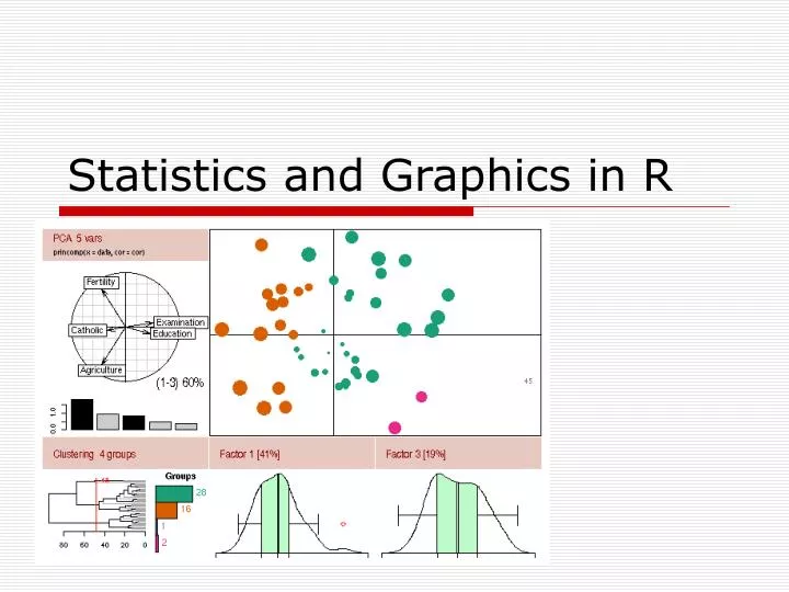
Statistics and Graphics in R. Barplot. y <- as.data.frame(matrix(runif(36), ncol=3, dimnames=list(month.abb, LETTERS[1:3]))) barplot(as.matrix(y[1:4,]), ylim=c(0,max(y[1:4,])+0.1), beside=T)

E N D
Barplot • y <- as.data.frame(matrix(runif(36), ncol=3, dimnames=list(month.abb, LETTERS[1:3]))) barplot(as.matrix(y[1:4,]), ylim=c(0,max(y[1:4,])+0.1), beside=T) text(x=seq(1.5, 13, by=1)+sort(rep(c(0,1,2), 4)), y=as.vector(as.matrix(y[1:4,]))+0.02,labels=round(as.vector(as.matrix(y[1:4,])),2)) • ysub <- as.matrix(y[1:4,]); myN <- length(ysub[,1]); mycol1 <- gray(1:(myN+1)/(myN+1))[-(myN+1)]; mycol2 <- sample(colors(),myN); barplot(ysub, beside=T, ylim=c(0,max(ysub)*1.2), col=mycol2, main="Bar Plot", sub="data: example"); legend("topright", legend=row.names(ysub), cex=1.3, bty="n", pch=15, pt.cex=1.8, col=mycol2, ncol=myN) • par(mar=c(10.1, 4.1, 4.1, 2.1)); par(xpd=TRUE); barplot(ysub, beside=T, ylim=c(0,max(ysub)*1.2), col=mycol2, main="Bar Plot"); legend(x=4.5, y=-0.6, legend=row.names(ysub), cex=1.3, bty="n", pch=15, pt.cex=1.8, col=mycol2, ncol=myN)
Barplot with Confidence Interval • stdev=data.frame(Sep.Len=tapply(iris[,1], iris$Species,sd), Sep.Wid =tapply(iris[,2], iris$Species,sd), Pet.Len=tapply(iris[,3], iris$Species,sd), Pet.Wid=tapply(iris[,4], iris$Species,sd) ) bar <- barplot(ysub, beside=T, ylim=c(0,max(ysub)*1.2), col=mycol2, main="Bar Plot") arrows(as.vector(bar), as.vector(ysub), as.vector(bar), as.vector(ysub)+ as.vector(as.matrix(stdev)), length=0.15, angle = 90); arrows(as.vector(bar), as.vector(ysub), as.vector(bar), as.vector(ysub)-as.vector(as.matrix(stdev)), length=0.15, angle = 90) legend("topright", legend=row.names(ysub), cex=1.3, bty="n", pch=15, pt.cex=1.8, col=mycol2, ncol=myN) • require(gplots) mybarcol <- “gray20”; ci.l <- as.matrix(ysub-stdev); ci.u <- as.matrix(ysub+stdev) mp <- barplot2(ysub, beside = TRUE,col = c("lightblue", "mistyrose","lightcyan"), legend = rownames(ysub), ylim = c(0, 10), main = "IRIS DataSet", font.main = 4, col.sub = mybarcol, cex.names = 1.5, plot.ci = TRUE, ci.l = ci.l, ci.u = ci.u,plot.grid = TRUE) mtext(side = 1, at = colMeans(mp), line = -2, text = paste("Mean", formatC(colMeans(ysub))), col = "red") box()
Pie Chart • y <- table(iris$Species) • pie(y, col=rainbow(length(y), start=0.1, end=0.8), main="Pie Chart", clockwise=T) # Plots a simple pie chart. • pie(y, col=rainbow(length(y), start=0.1, end=0.8), labels=NA, main="Pie Chart", clockwise=T); legend("topright", legend=row.names(y), cex=1.3, bty="n", pch=15, pt.cex=1.8, col=rainbow(length(y), start=0.1, end=0.8), ncol=1)
Plot Options • Multiple plots in a single graphic window par(mfrow=c(2,3)) #allows 6 plots to appear on a page (2 rows of 3 plots each) • Adjusting graphical parameters Types for plots and lines: type=“l“ (lines); type=“b“ (both); type=“o” (overstruck); type=“h” (high density) The line types using lty argument within plot() command; Colors and characters using col and pch argument • Putting text to the plot; controlling the text size y <- as.data.frame(matrix(runif(36), ncol=3, dimnames=list(month.abb, LETTERS[1:3]))) plot(y[,1], y[,2]) plot(y[,1], y[,2], type="n", main="Plot of Labels"); text(y[,1], y[,2], rownames(y)) plot(y[,1], y[,2], pch=20, col="red", main="Plot of Symbols and Labels"); text(y[,1]+0.03, y[,2], rownames(y)) # Plots both, symbols plus their labels.
Plot Options plot(y[,1:2], xlab=" ", ylab=" ", type="n") mtext("Text on side 1, cex=1", side=1,cex=1) mtext("Text on side 2, cex=1.2", side=2,cex=1.2) mtext("Text on side 3, cex=1.5", side=3,cex=1.5) mtext("Text on side 4, cex=2", side=4,cex=2) text(15, 4.3, "text(15, 4.3)") text(35, 3.5, adj=0, "text(35, 3.5), left aligned") text(40, 5, adj=1, "text(40, 5), right aligned")
Scatter Plots op <- par(mar=c(8,8,8,8), bg="lightblue"); plot(y[,1], y[,2], type="p", col="red", cex.lab=1.2, cex.axis=1.2, cex.main=1.2, cex.sub=1, lwd=4, pch=20, xlab="x label", ylab="y label", main="My Main", sub="My Sub"); par(op)
Scatter Plots • Adds a regression line and a mathematical formula to the plot myline <- lm(y[,2]~y[,1], data=y[,1:2]) plot(y[,1], y[,2]); text(y[1,1], y[1,2], expression(sum(frac(1,sqrt(x^2*pi)))), cex=1.3) abline(myline, lwd=2)
Scatterplot Matrices panel.cor <- function(x, y, digits=2, prefix="", cex.cor){ usr <- par("usr"); on.exit(par(usr)) par(usr = c(0, 1, 0, 1)) r <- abs(cor(x, y)) txt <- format(c(r, 0.123456789), digits=digits)[1] txt <- paste(prefix, txt, sep="") if(missing(cex.cor)) cex <- 0.8/strwidth(txt) text(0.5, 0.5, txt, cex = 1.3) } xy.panel <- function(x,y){ points(x,y,pch = 21, bg = c("red", "green3", "blue")[unclass(iris$Species)],cex=1.3) } pairs(iris[1:4], main = "Anderson's Iris Data -- 3 species",lower.panel=xy.panel, upper.panel=panel.cor)
Histogram hist(eruptions, seq(1.6, 5.2, 0.2), prob=T, col = gray(0.95)) lines(density(eruptions, bw=0.1)) rug(eruptions, side=1)
Bivariate Histogram library(UsingR) scatter.with.hist(faithful$eruptions,faithful$waiting)
Density Plots Overlayed Plots on One Graphic x=rnorm(100);y=rnorm(100) split.screen(c(2,1)); split.screen(c(1,2),screen=2) screen(3) plot(density(x), xlim=c(-2,2), ylim=c(0,1), col="red"); screen(4) plot(density(y), xlim=c(-2,2), ylim=c(0,1), col="blue"); screen(1) plot(density(x), xlim=c(-2,2), ylim=c(0,1), col="red"); screen(1, new=FALSE); plot(density(y), xlim=c(-2,2), ylim=c(0,1), col="blue", xaxt="n", yaxt="n", ylab="", xlab="", main="",bty="n"); axis(4) close.screen(all = TRUE)
Boxplots • y=rnorm(100) boxplot(y) # usual vertical boxplot boxplot(y, horizontal=T) # horizontal boxplot ; rug(y, side=1) • boxplot(Sepal.Length ~Species,data=iris) title(“Sepal length by IRIS Species”)
Perspective Plots persp(x, y, z, theta = 130, phi = 30, expand = 0.5, col = "lightblue", ltheta = -120, shade = 0.75, ticktype = "detailed", xlab = "X", ylab = "Y", zlab = "Sinc( r )" ) title(expression(z=Sinc(sqrt(x^2+y^2))))
3-dimensional Scatterplots library(scatterplot3d) scatterplot3d(iris[,1:3],color=c("red","blue","green")[iris$Species], col.axis="blue", col.grid ="lightblue", main ="scatterplot3d", pch=20,cex.symbols=2)
Some Extra Insights Feature Maps for DNA sequence plot(x <- rnorm(40,2e+07,sd=1e+07), y <- rep(1,times=40), type="h", col="blue", xaxt="n", yaxt="n", bty="n",xlab="",ylab=""); abline(h=0.78, col="green", lwd=12); lines(a <- rnorm(5,2e+07,sd=1e+07), b <- rep(1,times=5), type="h", col="red", lwd=2) text(locator(1), "Simulated chromosome maps")
Matrix Plots Confidence Interval m = 50; n=20; p = .5; # toss 20 coins 50 times phat = rbinom(m,n,p)/n # divide by n for proportions SE = sqrt(phat*(1-phat)/n) # compute SE alpha = 0.10;zstar = qnorm(1-alpha/2) matplot(rbind(phat - zstar*SE, phat + zstar*SE),rbind(1:m,1:m),type="l",lty=1) abline(v=p)
Saving Graphics to Files • jpeg("test.jpeg"); plot(1:10, 1:10); dev.off() # After the 'jpeg("test.jpeg")' command all graphs are redirected to the file "test.jpeg" in JPEG format. To export images with the highest quality, the default setting "quality = 75" needs to be changed to 100%. The actual image data are not written to the file until the 'dev.off()' command is executed! • pdf("test.pdf"); plot(1:10, 1:10); dev.off() # Same as above, but for pdf format. The pdf format provides often the best image quality, since it scales to any size without pixelation. • png("test.png"); plot(1:10, 1:10); dev.off() # Same as above, but for png format. • postscript("test.ps"); plot(1:10, 1:10); dev.off() # Same as above, but for PostScript format.
Statistical models in R The operator ~ is used to define a model formula in R. The form, for an ordinary linear model, is response ~ op_1 term_1 op_2 term_2 op_3 term_3 ... where response is a vector or matrix, (or expression evaluating to a vector or matrix) defining the response variable(s). op_i : an operator, either + or -, implying the inclusion or exclusion of a term in the model, (the first is optional). term_i : is either a vector or matrix expression, or 1, a factor, or a formula expression consisting of factors, vectors or matrices connected by formula operators. In all cases each term defines a collection of columns either to be added to or removed from the model matrix. A 1 stands for an intercept column and is by default included in the model matrix unless explicitly removed.
Example • y ~ x - 1 #Simple linear regression of y on x through the origin (that is, without an intercept term). • log(y) ~ x1 + x2 # Multiple regression of the transformed variable, log(y), on x1 and x2 (with an implicit intercept term). • y ~ poly(x,2) ; y ~ 1 + x + I(x^2) #Polynomial regression of y on x of degree 2. The first form uses orthogonal polynomials, and the second uses explicit powers, as basis. • y ~ X + poly(x,2) #Multiple regression y with model matrix consisting of the matrix X as well as polynomial terms in x to degree 2. • y ~ A #Single classification analysis of variance model of y, with classes determined by A. • y ~ A + x #Single classification analysis of covariance model of y, with classes determined by A, and with covariate x. • y ~ A*B ; y ~ A + B + A:B ; y ~ B %in% A ; y ~ A/B #Two factor non-additive model of y on A and B. The first two specify the same crossed classification and the second two specify the same nested classification. In abstract terms all four specify the same model subspace.
Example • y ~ (A + B + C)^2 ; y ~ A*B*C - A:B:C #Three factor experiment but with a model containing main effects and two factor interactions only. Both formulae specify the same model. • y ~ A * x ; y ~ A/x ; y ~ A/(1 + x) - 1 #Separate simple linear regression models of y on x within the levels of A, with different codings. The last form produces explicit estimates of as many different intercepts and slopes as there are levels in A. • y ~ A*B + Error(C) #An experiment with two risk factors, A and B, and error strata determined by factor C. For example a split plot experiment, with whole plots (and hence also subplots), determined by factor C.
Linear Model ctl <- c(4.17,5.58,5.18,6.11,4.50,4.61,5.17,4.53,5.33,5.14) trt <- c(4.81,4.17,4.41,3.59,5.87,3.83,6.03,4.89,4.32,4.69) group <- gl(2,10,20, labels=c("Ctl","Trt")) weight <- c(ctl, trt) anova(fm1 <- lm(weight ~ group)) ; summary(fm2 <- lm(weight ~ group - 1))# omitting intercept summary(resid(fm1) - resid(fm2))
Generic functions for extracting model information • The value of lm() is a fitted model object; technically a list of results of class "lm". Generic functions that orient themselves to objects of class "lm“ include, add1 deviance formula predict step alias drop1 kappa print summary anova effects labels proj vcov coef family plot residuals • anova(object_1, object_2) Compare two or more models and produce an analysis of variance table. • coef(object) Extract the regression coefficient (matrix). • deviance(object) Residual sum of squares, weighted if appropriate.
Generic functions for extracting model information (Cont’d) • formula(object) Extract the model formula. • plot(object) Produce four plots, showing residuals, fitted values and some diagnostics. • predict(object, newdata=data.frame) The data frame supplied must have variables specified with the same labels as the original. The value is a vector or matrix of predicted values corresponding to the determining variable values in data.frame. • residuals(object) Extract the (matrix of) residuals, weighted as appropriate. • step(object) Select a suitable model by adding or dropping terms and preserving hierarchies. The model with the smallest value of AIC (Akaike's An Information Criterion) discovered in the stepwise search is returned. • summary(object) Print a comprehensive summary of the results of the regression analysis. • vcov(object) Returns the variance-covariance matrix of the main parameters of a fitted model object.
Generalized linear models • There is a response, y, of interest and stimulus variables x_1, x_2, ..., whose values influence the distribution of the response. The stimulus variables influence the distribution of y through a single linear function, only. This linear function is called the linear predictor, and is usually written eta = beta_1 x_1 + beta_2 x_2 + ... + beta_p x_p, hence x_i has no influence on the distribution of y if and only if beta_i is zero. • The distribution of y is of the form f_Y(y; mu, phi) = exp((A/phi) * (y lambda(mu) - gamma(lambda(mu))) + tau(y, phi)), where phi is a scale parameter (possibly known), and is constant for all observations, A represents a prior weight, assumed known but possibly varying with the observations, and mu is the mean of y. So it is assumed that the distribution of y is determined by its mean and possibly a scale parameter as well. • The mean, mu, is a smooth invertible function of the linear predictor: mu = m(eta), eta = m^{-1}(mu) = ell(mu) and this inverse function, ell(), is called the link function.
Families and Link Functions on GLM Family name Link functions binomial logit, probit, log, cloglog gaussian identity, log, inverse Gamma identity, inverse, log inverse.gaussian 1/mu^2, identity, inverse, log poisson identity, log, sqrt quasi logit, probit, cloglog, identity, inverse, log, 1/mu^2, sqrt
GLM Function • The R function to fit a generalized linear model is glm() which uses the form > fitted.model <- glm(formula, family=family.generator, data=data.frame) • To fit a binomial model using glm() there are three possibilities for the response: If the response is a vector it is assumed to hold binary data, and so must be a 0/1 vector. If the response is a two-column matrix it is assumed that the first column holds the number of successes for the trial and the second holds the number of failures. If the response is a factor, its first level is taken as failure (0) and all other levels as `success' (1). • kalythos <- data.frame(x = c(20,35,45,55,70), n = rep(50,5), y = c(6,17,26,37,44)) kalythos$Ymat <- cbind(kalythos$y, kalythos$n - kalythos$y) fmp <- glm(Ymat ~ x, family = binomial(link=probit), data = kalythos) fml <- glm(Ymat ~ x, family = binomial, data = kalythos) #logit link is the default summary(fmp); summary(fml)
Other Statistics Model in R • Mixed models. The recommended nlme package provides functions lme() and nlme() for linear and non-linear mixed-effects models. • Local approximating regressions. The loess() function fits a nonparametric regression by using a locally weighted regression. Function loess is in the standard package stats, together with code for projection pursuit regression ppr(). • Robust regression. There are several functions available for fitting regression models in a way resistant to the influence of extreme outliers in the data. Function lqs in the recommended package MASS provides state-of-art algorithms for highly-resistant fits. Less resistant but statistically more efficient methods are available in packages, for example function rlm in package MASS. • Additive models. This technique aims to construct a regression function from smooth additive functions of the determining variables, usually one for each determining variable. Functions avas and ace in package acepack and functions bruto and mars in package mda provide some examples of these techniques in user-contributed packages to R. An extension is Generalized Additive Models, implemented in user-contributed packages gam and mgcv. • Tree-based models. Tree-based models seek to bifurcate the data, recursively, at critical points of the determining variables in order to partition the data ultimately into groups that are as homogeneous as possible within, and as heterogeneous as possible between. The tree model can be implemented in packages rpart and tree.