Download
1 / 38
380 likes | 382 Views
Explore the scientific consensus on climate change, new research directions, and the implications for policy. Learn about global warming, greenhouse gases, impacts on ecosystems, and regional climate modeling. Discover the effects on sea ice, glaciers, precipitation patterns, vegetation distribution, and sea level rise. Understand the potential consequences for agriculture and wine regions.

E N D
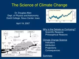
The Science of Climate Change Scientific Consensus, New Research Directions, and Implications for Policy Prof. Alex Hall UCLA Department of Atmospheric and Oceanic Sciences
Data: Surface Warming Global mean surface warming 1900 to 2000: 0.6 °C (IPCC 2001, Jones et al. 1999)
CO2 isn’t the only human-related factor affecting climate. Slightly less than half the human enhancement of the greenhouse effect is caused by other gases, including methane and nitrous oxide. Also, aerosols have a large and difficult to quantify impact on climate.
Computational grid of a general circulation model This is the typical resolution of a climate model. Note that there are many important processes for climate (such as those related to cloud), that cannot be resolved explicitly on such a coarse grid. Note also that the most relevant climate impacts are not simulated at this resolution.
Modeled and Predicted Temperatures Tett et al., 1999
SURFACE ALBEDO FEEDBACK Surface albedo feedback is thought to be a positive feedback mechanism. Its effect is strongest in mid to high latitudes, where there is significant coverage of snow and sea ice. Increase in temperature Increase in incoming sunshine Decrease in sea ice and snow cover
Northern hemisphere snow cover is decreasing. (Armstrong and Brodzik 1999). The rate is equivalent to losing an area the size of California every 7 years.
Arctic researchers see early warming signals 1979 2000 Based on satellite data, these images show Arctic sea ice. The ice cover shrunk by 9 percent a decade over that time.
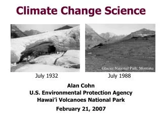
1938 1981 Grinnell Glacier Glacier National Park Loss of Mountain Glaciers
Mountain glaciers all over the world are in retreat. This is the Qori Kalis glacier in Peru in 1978. Here is the same glacier in the year 2000. The lake covers 10 acres.
From space, we can monitor the extent of melting of the world’s major ice sheets. Greenland has experienced a large increase in melting over the past few decades. Images courtesy of Konrad Steffen and Russell Huff, CIRES, University of Colorado at Boulder
There are two main global effects associated with climate change: (1) An increase in global mean temperature, which we have discussed already. (2) An increase in evaporation everywhere, driven by increased greenhouse gas concentrations and increased temperatures. The increase in evaporation also implies an increase in precipitation, because the atmosphere can’t store water vapor indefinitely. There is no clear consensus on how the increase in precipitation will be distributed. However, we do know that it will not be distributed uniformly. This increase in evaporation and precipitation is known as the intensification of the hydrologic cycle.
The change in distribution of precipitation will have a significant effect on total biomass. This of course will also affect species composition and diversity significantly. Some of these effects can be estimated by coupling vegetation models to global climate models during climate change experiments. This plot shows the change in simulated total live vegetation (biomass) between last decade of the 21st century and 1961-1990 from two different climate models (Bachelet et al. 2001)
One easilyanticipated effect of climate change isspecies migrationto higher latitudes.For example, a warmer climate may have significant effect on forests composition. Decidous forests will probably move northwards and to higher altitudes, replacing coniferous forests in many areas. Some tree species will probably be replaced altogether, jeopardizing biological diversity.
HadCM3 higher HadCM3 lower PCM higher PCM lower Changes in Vegetation Distribution2070-2099, relative to 1961-1990 Temperature-driven Fire-mediated Source: A Luers/Union of Concerned Scientists
About 2/3 of the observed sea level rise is probably attributable to thermal expansion of seawater; the remainder is due to melting of glaciers
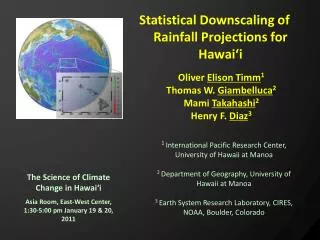
april annual significance temperature increase snow loss Regional climate modeling is a promising approach to give detail necessary to discuss impacts.
Diminishing Sierra Snowpack% Remaining, Relative to 1961-1990 Higher Emissions Lower Emissions Source: A Luers/Union of Concerned Scientists
Decreasing Wine Grape QualityTemperature Impacts LOWER EMISSIONS HIGHER EMISSIONS Wine Country (Sonoma, Napa Counties) Cool Coastal (Mendocino, Monterey Counties) Northern Central Valley (San Joaquin, Sacramento Counties) Source: A Luers/Union of Concerned Scientists
A view of the Santa Anas from space, taken by the Multi-angle Imaging SpectroRadiometer (MISR) on February 9, 2002.
The winds simulated by the model during the Santa Ana event of February 9-12, 2002. Note the intense flow, reaching speeds on the order of 10 meters per second, being channeled through mountain passes.
CREATING CHANGE International, National, or Local? Public Opinion Science Research Interest Groups