Download
1 / 26
270 likes | 354 Views
The launch and collimation …. Stellar jets transport significant amounts of energy and momentum away from the powering source important role in its evolution. The jet production mechanism works on very small spatial scales the central jet engine is often heavily embedded.

E N D
Stellar jets transport significant amounts of energy and momentum away from the powering source important role in its evolution. The jet production mechanism works on very small spatial scales the central jet engine is often heavily embedded Many open questions remain to be resolved, eg, the nature of the accretion/ejection relationship the jet generation mechanims whether the process is similar on all masses and length scales
Models of jet generation It is widely accepted that to make a fast collimated jet requiured: accretion disk large-scale magnetic field. This is because neither gas pressure nor radiation pressure are enough to collimate large momentum flux. MAGNETO-CENTRIFUGAL MODELS: During the accretion process, magneto-centrifugal forces are responsible for launch acceleration of the stellar jet collimation
Observational challenges Main observational difficulties in testing models lie: YSO are heavily embedded Infall and outflow kinematics are complex and confused close to the source Spatial and temporal scales ar relatively small. Ex: considering the length scales involved for Taurus (d~140 pc): Jet acceleration and collimation zone ~ 1-40 AU above the plane of disk 0.1” res. Jet engine operates on sclales of < 5 AU 0.01” res. Observational difficulties persit even the jet has travelled far from the source: emission lines mark the location of shock fronts and post-shock cooling zone (length scales ~ tens AU) Jet widths are typically ~ 15 AU Hence, resolving the jet internal structure, excitation and kinematics is heavily dependent on high spatial resolution data
The region of the jet launch Outflows are ultimately powered by the release of Eg liberated by accretion onto the YSO ( only ~ 10% ; the rest is radiated). It is likely that the acceleration of an outflow and its collimation occur at different location and involving different processes: Most outflow are probably launched at radii of at most a few AU , while Most jets have beams ~50-500 AU wide at the point where they first become visible Indication that collimation occurs at larger distances from the source than the launch region.
Collimation l>>w Need to determine the jet width as close as possible to the powering source Ideally: at a few R* 1012cm 0.5mas for a d~140pc (Taurus) “Problems”: +Observation:limited by the spatial resolution. +Intrinsec: * Powering source, deeply embedded high optical/ir extinction jet are observed beginning from few arcsec from the powering source. *Light reflected by the disk produces a bright background ( low contrast) that makes difficult to measure the jet width.
Case A : jet collimation “far” from the source Case B:jet collimation “close” to the source Mundt & Raga: ai= mean jet aperture inside the box aa=mean jet aperture outside the box Measured in 15 jets: ai 0 a 3º ai>3aa Seems to favour Case A “Forbidden observing box” 0.5-10” (70-1500AU)
MECHANISMS OF COLLIMATION OF THE JET Currently, there are three main magnetohydrodynamic (MHD) models, which differ mainly in the origin of magnetic forces which drive the jet: 1.- The stellar wind 2.-The X-wind 3.- The Disk-wind
The Stellar wind model The jet launching point is the stellar surface PROBLEMS: Difficulties in achieving sufficient angular momentum extraction to slow the stellar rotation to the observed via stellar wind alone.
The X-Wind model The magnetic X-point (point where the stellar magnetosphere intersects the disk) is the point of origin of a magneto-centrifugally driven wind, fueled by matter injected onto the open field lines. The magnetic forces on the open field lines, at scales of ~ 0.03 AU from the source, are responsible for collimating the wind into a jet
The Disk-wind model Centrifugally driven winds are launched from a magnetised disk surface launch occurs not only close to the source, but also up to a few AU along the disk (~0.03 to 5 AU)
Knots: steady crossing-shocks (model from Raga, Cantó) A jet which initially has a pressure higher than the environment, expands freely until its pressure falls below the pressure of the ambient It is then recollimated by a curved “incident shock” Where the incident shock converges on the jet axis, it sets up a “reflected shock” Since it is now again overpressured compared to its environment, it will Expand and the whole pattern is repeated.
Advantadges: Makes possible to extensively explore parameter space. Predict the jet appearance in various emission lines and calculate theoretical long-slit spectra. Problems: Not very realistic, eg, If the observed knots are identified with the predicted crossing-shock cells, the observed length-to-width ratio is an order of magnitude smaller than the calculated (~1.4 x Mj; Mj~20; Mj, Mach number). Observed proper motion cannot be reproduced in these stationary models.
** Jets: knots/interknots discontinuous intensity Knotscrossing shocks qM=sin-1(aT/Vj) qM= Mach angle aT=sound velocity Vj=jet velocity Differences between pj y pe give rise to a pair of shock waves (incident/reflected) Problems:stationary knots
SHOCK MODELS IN HHs HHs: Observational signature of the shock produced by the collision of two fluids with their velocities ranging 10 -- 300 km/s Models: plausible scenarios 1.- Internal shocks within a moving fluid (jet or wind) 2.-Entrainment of dense gas by jet or wind. 3.- Bow-shock produced when the wind is intersected by an obstacle. 4.- A dense knot (“bullet”) goes through an obstacle. (Models 2 and 4 are similar, except in the relationship between the densities of the high-velocity and stationary gas).
Schematic diagram showing a two-shock working surfaceformed by the interaction of a flow ofhigh velocity V2with a previously ejected flow of slower velocity V1.The working surface moves with anintermediate velocity Vws. Shock Vws V1 V2 v Shock Velocity variations Variabilities in the ejection velocity results in the generation ofinternal “working surfaces” as the high velocity sections of the flow catches up the slow ones previously ejected.
The working surface of a jet Two fluid colliding supersonically: two shocks are generated: 1.- a shock in which material from the environment is accelerated bow-shock 2.- a shock in which the jet material is decelerated jet shock The whole double shock structure is the working surface The shocks are separated by a contact discontinuity
Structure of the working surface Incident jet gas (r1, v1) encounters gas (r2,v2 < v1). Impact occurs at the Mach disk, also known at the jet shock. Gas traversing this front creates the curved bow-shock on the right. In between the two fronts, material spills out laterally, forming the cocoon The widest bow-shocks observed have a clumpy morphology and display short-temporal fluctuations: The inter-shock material is not an homogeneous fluid: two flows with distinct properties enter and are unlikely to mix completely. The weaker Shock, at lower temperature, cools more rapidly, forms a dense shell. Breaks as fresh material joins it.
Models: density maps of the working surface after 800 yr (a) and 1200 yr (b)
Spatial non-coincidence of the emission from different lines