Download
1 / 56
560 likes | 673 Views
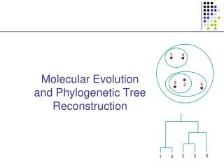
Phylogenetic reconstruction, probability mapping, types of selection. Peter Gogarten Office: BSP 404 phone: 860 486-4061, Email: gogarten@uconn.edu. Sequence alignment:. CLUSTALW. MUSCLE. Removing ambiguous positions:. T-COFFEE. FORBACK. Generation of pseudosamples:. SEQBOOT.

E N D
Phylogenetic reconstruction, probability mapping,types of selection. Peter Gogarten Office: BSP 404 phone: 860 486-4061, Email:gogarten@uconn.edu
Sequence alignment: CLUSTALW MUSCLE Removing ambiguous positions: T-COFFEE FORBACK Generation of pseudosamples: SEQBOOT PROTDIST TREE-PUZZLE Calculating and evaluating phylogenies: PROTPARS PHYML NEIGHBOR FITCH SH-TEST in TREE-PUZZLE CONSENSE Comparing phylogenies: Comparing models: Maximum Likelihood Ratio Test Visualizing trees: ATV, njplot, or treeview Phylip programs can be combined in many different ways with one another and with programs that use the same file formats.
Elliot Sober’s Gremlins Observation: Loud noise in the attic ? Hypothesis: gremlins in the attic playing bowling Likelihood = P(noise|gremlins in the attic) P(gremlins in the attic|noise) ? ?
TreePuzzle ne PUZZLE TREE-PUZZLE is a very versatile maximum likelihood program that is particularly useful to analyze protein sequences. The program was developed by Korbian Strimmer and Arnd von Haseler (then at the Univ. of Munich) and is maintained by von Haseler, Heiko A. Schmidt, and Martin Vingron (contacts see http://www.tree-puzzle.de/).
TREE-PUZZLE • allows fast and accurate estimation of ASRV (through estimating the shape parameter alpha) for both nucleotide and amino acid sequences, • It has a “fast” algorithm to calculate trees through quartet puzzling (calculating ml trees for quartets of species and building the multispecies tree from the quartets). • The program provides confidence numbers (puzzle support values), which tend to be smaller than bootstrap values (i.e. provide a more conservative estimate), • the program calculates branch lengths and likelihood for user defined trees, which is great if you want to compare different tree topologies, or different models using the maximum likelihood ratio test. • Branches which are not significantly supported are collapsed. • TREE-PUZZLE runs on "all" platforms • TREE-PUZZLE reads PHYLIP format, and communicates with the user in a way similar to the PHYLIP programs.
Maximum likelihood ratio test If you want to compare two models of evolution (this includes the tree) given a data set, you can utilize the so-called maximum likelihood ratio test. If L1 and L2 are the likelihoods of the two models, d =2(logL1-logL2) approximately follows a Chi square distribution with n degrees of freedom. Usually n is the difference in model parameters. I.e., how many parameters are used to describe the substitution process and the tree. In particular n can be the difference in branches between two trees (one tree is more resolved than the other). In principle, this test can only be applied if on model is a more refined version of the other. In the particular case, when you compare two trees, one calculated without assuming a clock, the other assuming a clock, the degrees of freedom are the number of OTUs – 2 (as all sequences end up in the present at the same level, their branches cannot be freely chosen) . To calculate the probability you can use the CHISQUARE calculator for windows available from Paul Lewis.
TREE-PUZZLE allows (cont) • TREEPUZZLE calculates distance matrices using the ml specified model. These can be used in FITCH or Neighbor. • PUZZLEBOOT automates this approach to do bootstrap analyses – WARNING: this is a distance matrix analyses! • The official script for PUZZLEBOOT is here – you need to create a command file (puzzle.cmds), and puzzle needs to be envocable through the command puzzle. • Your input file needs to be the renamed outfile from seqboot • A slightly modified working version of puzzleboot_mod.sh is here, and here is an example for puzzle.cmds . Read the instructions before you run this! • Maximum likelihood mapping is an excellent way to • assess the phylogenetic information contained in a dataset. • ML mapping can be used to calculate the support around one branch. • @@@ Puzzle is cool, don't leave home without it! @@@
P(data|model, I) P(model|data, I) = P(model, I) P(data,I) Likelihood describes how well the model predicts the data Bayes’ Theorem Posterior Probability represents the degree to which we believe a given model accurately describes the situation given the available data and all of our prior information I Prior Probability describes the degree to which we believe the model accurately describes reality based on all of our prior information. Normalizing constant Reverend Thomas Bayes (1702-1761)
Li pi= L1+L2+L3 Ni pi Ntotal Alternative Approaches to Estimate Posterior Probabilities Bayesian Posterior Probability Mapping with MrBayes(Huelsenbeck and Ronquist, 2001) Problem: Strimmer’s formula only considers 3 trees (those that maximize the likelihood for the three topologies) Solution: Exploration of the tree space by sampling trees using a biased random walk (Implemented in MrBayes program) Trees with higher likelihoods will be sampled more often ,where Ni - number of sampled trees of topology i, i=1,2,3 Ntotal – total number of sampled trees (has to be large)
ml mapping From: Olga Zhaxybayeva and J Peter Gogarten BMC Genomics 2002, 3:4
ml mapping Figure 5. Likelihood-mapping analysis for two biological data sets. (Upper) The distribution patterns. (Lower) The occupancies (in percent)for the seven areas of attraction. (A) Cytochrome-b data fromref. 14. (B) Ribosomal DNA of major arthropod groups (15). From: Korbinian Strimmer and Arndt von HaeselerProc. Natl. Acad. Sci. USAVol. 94, pp. 6815-6819, June 1997
ml mapping (cont) If we want to know if Giardia lamblia forms the deepest branch within the known eukaryotes, we can use ML mapping to address this problem. To apply ml mapping we choose the "higher" eukaryotes as cluster a, another deep branching eukaryote (the one that competes against Giardia) as cluster b, Giardia as cluster c, and the outgroup as cluster d. For an example output see this sample ml-map. An analysis of the carbamoyl phosphate synthetase domains with respect to the root of the tree of life is here. Application of ML mapping to comparative Genome analyses see here for a comparison of different probability measures see here for an approach that solves the problem of poor taxon sampling that is usually considered inherent with quartet analyses is.
(a,b)-(c,d) /\ / \ / \ / 1 \ / \ / \ / \ / \ / \/ \ / 3 : 2 \ / : \ /__________________\ (a,d)-(b,c) (a,c)-(b,d)Number of quartets in region 1: 68 (= 24.3%)Number of quartets in region 2: 21 (= 7.5%)Number of quartets in region 3: 191 (= 68.2%)Occupancies of the seven areas 1, 2, 3, 4, 5, 6, 7: (a,b)-(c,d) /\ / \ / 1 \ / \ / \ / /\ \ / 6 / \ 4 \ / / 7 \ \ / \ /______\ / \ / 3 : 5 : 2 \ /__________________\ (a,d)-(b,c) (a,c)-(b,d)Number of quartets in region 1: 53 (= 18.9%) Number of quartets in region 2: 15 (= 5.4%) Number of quartets in region 3: 173 (= 61.8%) Number of quartets in region 4: 3 (= 1.1%) Number of quartets in region 5: 0 (= 0.0%) Number of quartets in region 6: 26 (= 9.3%) Number of quartets in region 7: 10 (= 3.6%) Cluster a: 14 sequencesoutgroup (prokaryotes) Cluster b: 20 sequencesother Eukaryotes Cluster c: 1 sequencesPlasmodium Cluster d: 1 sequences Giardia
P(data|model, I) P(model|data, I) = P(model, I) P(data,I) Likelihood describes how well the model predicts the data Bayes’ Theorem Posterior Probability represents the degree to which we believe a given model accurately describes the situation given the available data and all of our prior information I Prior Probability describes the degree to which we believe the model accurately describes reality based on all of our prior information. Normalizing constant Reverend Thomas Bayes (1702-1761)
Illustration of a biased random walk Figure generated using MCRobot program (Paul Lewis, 2001)
Li pi= L1+L2+L3 Ni pi Ntotal Alternative Approaches to Estimate Posterior Probabilities Bayesian Posterior Probability Mapping with MrBayes(Huelsenbeck and Ronquist, 2001) Problem: Strimmer’s formula only considers 3 trees (those that maximize the likelihood for the three topologies) Solution: Exploration of the tree space by sampling trees using a biased random walk (Implemented in MrBayes program) Trees with higher likelihoods will be sampled more often ,where Ni - number of sampled trees of topology i, i=1,2,3 Ntotal – total number of sampled trees (has to be large)
COMPARISON OF DIFFERENT SUPPORT MEASURES A: mapping of posterior probabilities according to Strimmer and von Haeseler B: mapping of bootstrap support values C: mapping of bootstrap support values from extended datasets Zhaxybayeva and Gogarten, BMC Genomics 2003 4: 37
bootstrap values from extended datasets More gene families group species according to environment than according to 16SrRNA phylogeny In contrast, a themophilic archaeon has more genes grouping with the thermophilic bacteria ml-mapping versus
the gradualist point of view Evolution occurs within populations where the fittest organisms have a selective advantage. Over time the advantages genes become fixed in a population and the population gradually changes. Note: this is not in contradiction to the the theory of neutral evolution. (which says what ?) • Processes that MIGHT go beyond inheritance with variation and selection? • Horizontal gene transfer and recombination • Polyploidization (botany, vertebrate evolution) see here • Fusion and cooperation of organisms (Kefir, lichen, also the eukaryotic cell) • Targeted mutations (?), genetic memory (?) (see Foster's and Hall's reviews on directed/adaptive mutations; see here for a counterpoint) • Random genetic drift • Gratuitous complexity • Selfish genes (who/what is the subject of evolution??) • Parasitism, altruism, Morons
selection versus drift see Kent Holsinger’s java simulations at http://darwin.eeb.uconn.edu/simulations/simulations.html The law of the gutter. compare drift versus select + drift The larger the population the longer it takes for an allele to become fixed. Note: Even though an allele conveys a strong selective advantage of 10%, the allele has a rather large chance to go extinct. Note#2: Fixation is faster under selection than under drift. BUT
s=0 Probability of fixation, P, is equal to frequency of allele in population. Mutation rate (per gene/per unit of time) = u ; freq. with which allele is generated in diploid population size N =u*2N Probability of fixation for each allele = 1/(2N) Substitution rate = frequency with which new alleles are generated * Probability of fixation= u*2N *1/(2N) = u Therefore: If f s=0, the substitution rate is independent of population size, and equal to the mutation rate !!!! (NOTE: Mutation unequal Substitution! )This is the reason that there is hope that the molecular clock might sometimes work. Fixation time due to drift alone: tav=4*Ne generations (Ne=effective population size; For n discrete generations Ne= n/(1/N1+1/N2+…..1/Nn)
s>0 Time till fixation on average: tav= (2/s) ln (2N) generations (also true for mutations with negative “s” ! discuss among yourselves) E.g.: N=106, s=0: average time to fixation: 4*106 generationss=0.01: average time to fixation: 2900 generations N=104, s=0: average time to fixation: 40.000 generationss=0.01: average time to fixation: 1.900 generations => substitution rate of mutation under positive selection is larger than the rate with which neutral mutations are fixed.
Random Genetic Drift Selection 100 advantageous Allele frequency disadvantageous 0 Modified from from www.tcd.ie/Genetics/staff/Aoife/GE3026/GE3026_1+2.ppt
Positive selection • A new allele (mutant) confers some increase in the fitness of the organism • Selection acts to favour this allele • Also called adaptive selection or Darwinian selection. NOTE: Fitness = ability to survive and reproduce Modified from from www.tcd.ie/Genetics/staff/Aoife/GE3026/GE3026_1+2.ppt
Advantageous allele Herbicide resistance gene in nightshade plant Modified from from www.tcd.ie/Genetics/staff/Aoife/GE3026/GE3026_1+2.ppt
Negative selection • A new allele (mutant) confers some decrease in the fitness of the organism • Selection acts to remove this allele • Also called purifying selection Modified from from www.tcd.ie/Genetics/staff/Aoife/GE3026/GE3026_1+2.ppt
Deleterious allele Human breast cancer gene, BRCA2 5% of breast cancer cases are familial Mutations in BRCA2 account for 20% of familial cases Normal (wild type) allele Mutant allele (Montreal 440 Family) Stop codon 4 base pair deletion Causes frameshift Modified from from www.tcd.ie/Genetics/staff/Aoife/GE3026/GE3026_1+2.ppt
Neutral mutations • Neither advantageous nor disadvantageous • Invisible to selection (no selection) • Frequency subject to ‘drift’ in the population • Random drift – random changes in small populations
Types of Mutation-Substitution • Replacement of one nucleotide by another • Synonymous (Doesn’t change amino acid) • Rate sometimes indicated by Ks • Rate sometimes indicated by ds • Non-Synonymous (Changes Amino Acid) • Rate sometimes indicated by Ka • Rate sometimes indicated by dn (this and the following 4 slides are from mentor.lscf.ucsb.edu/course/ spring/eemb102/lecture/Lecture7.ppt)
Genetic Code – Note degeneracy of 1st vs 2nd vs 3rd position sites
Genetic Code Four-fold degenerate site – Any substitution is synonymous From: mentor.lscf.ucsb.edu/course/spring/eemb102/lecture/Lecture7.ppt
Genetic Code Two-fold degenerate site – Some substitutions synonymous, some non-synonymous From: mentor.lscf.ucsb.edu/course/spring/eemb102/lecture/Lecture7.ppt
Measuring Selection on Genes • Null hypothesis = neutral evolution • Under neutral evolution, synonymous changes should accumulate at a rate equal to mutation rate • Under neutral evolution, amino acid substitutions should also accumulate at a rate equal to the mutation rate From: mentor.lscf.ucsb.edu/course/spring/eemb102/lecture/Lecture7.ppt
Counting #s/#a Ser Ser Ser Ser Ser Species1 TGA TGC TGT TGT TGT Ser Ser Ser Ser Ala Species2 TGT TGT TGT TGT GGT #s = 2 sites #a = 1 site #a/#s=0.5 To assess selection pressures one needs to calculate the rates (Ka, Ks), i.e. the occurring substitutions as a fraction of the possible syn. and nonsyn. substitutions. Things get more complicated, if one wants to take transition transversion ratios and codon bias into account. See chapter 4 in Nei and Kumar, Molecular Evolution and Phylogenetics. Modified from: mentor.lscf.ucsb.edu/course/spring/eemb102/lecture/Lecture7.ppt
Low number of polymorphisms Other approaches: A selective sweep decreases the number of polymorphisms present in a population surrounding the gene that was driven into fixation due to positive selection. This provides an alternative to dN/dS ratios to detect genes under positive selection. Number of non-synonymous substitutions large dN If a site or a gene repeatedly was driven into fixation due to positive selection, its substitution rate will be higher than the mutation rate. This diversifying selection is frequently observed for sites interacting with immune system.
dambe Two programs worked well for me to align nucleotide sequences based on the amino acid alignment, One is DAMBE (only for windows). This is a handy program for a lot of things, including reading a lot of different formats, calculating phylogenies, it even runs codeml (from PAML) for you. The procedure is not straight forward, but is well described on the help pages. After installing DAMBE go to HELP -> general HELP -> sequences -> align nucleotide sequences based on …-> If you follow the instructions to the letter, it works fine. DAMBE also calculates Ka and Ks distances from codon based aligned sequences.
aa based nucleotide alignments (cont) An alternative is the tranalign program that is part of the emboss package. On bbcxsrv1 you can invoke the program by typing tranalign. Instructions and program description are here . If you want to use your own dataset in the lab on Friday, generate a codon based alignment with either dambe or tranalign and save it as a nexus file and as a phylip formated multiple sequence file (using either clustalw, PAUP (export or tonexus), dambe, or readseq on the web)
sites versus branches You can determine omega for the whole dataset; however, usually not all sites in a sequence are under selection all the time. PAML (and other programs) allow to either determine omega for each site over the whole tree, , or determine omega for each branch for the whole sequence, . It would be great to do both, i.e., conclude codon 176 in the vacuolar ATPases was under positive selection during the evolution of modern humans – alas, a single site does not provide any statistics ….
Sites model(s) work great have been shown to work great in few instances. The most celebrated case is the influenza virus HA gene. A talk by Walter Fitch (slides and sound) on the evolution ofthis molecule is here . This article by Yang et al, 2000 gives more background on ml aproaches to measure omega. The dataset used by Yang et al is here: flu_data.paup .
sites model in MrBayes The MrBayes block in a nexus file might look something like this: begin mrbayes; set autoclose=yes; lset nst=2 rates=gamma nucmodel=codon omegavar=Ny98; mcmcp samplefreq=500 printfreq=500; mcmc ngen=500000; sump burnin=50; sumt burnin=50; end;
Vincent Daubin and Howard Ochman: Bacterial Genomes as New Gene Homes: The Genealogy of ORFans in E. coli. Genome Research 14:1036-1042, 2004 The ratio of non-synonymous to synonymous substitutions for genes found only in the E.coli - Salmonella clade is lower than 1, but larger than for more widely distributed genes. Fig. 3 from Vincent Daubin and Howard Ochman, Genome Research 14:1036-1042, 2004
Trunk-of-my-car analogy: Hardly anything in there is the is the result of providing a selective advantage. Some items are removed quickly (purifying selection), some are useful under some conditions, but most things do not alter the fitness. Could some of the inferred purifying selection be due to the acquisition of novel detrimental characteristics (e.g., protein toxicity)?
where to get help read the manuals and help files check out the discussion boards at http://www.rannala.org/phpBB2/ else there is a new program on the block called hy-phy(=hypothesis testing using phylogenetics). The easiest is probably to run the analyses on the authors datamonkey.
hy-phy Results of an anaylsis using the SLAC approach
Hy-Phy -Hypothesis Testing using Phylogenies. Using Batchfiles or GUI Information at http://www.hyphy.org/ Selected analyses also can be performed online at http://www.datamonkey.org/
Example testing for dN/dS in two partitions of the data --John’s dataset Set up two partitions, define model for each, optimize likelihood
Example testing for dN/dS in two partitions of the data --John’s dataset Safe Likelihood Function thenselect as alternative The dN/dS ratios for the two partitions are different.