Download
1 / 103
1.24k likes | 1.53k Views
Chapter 10: Climate Modeling. (Ch. 10, p. 254–285) Why use models? What models are available? Why simple models? History development of climate models How to evaluate models? Climate models in IPCC AR4 Example: NCAR CCSM

E N D
Chapter 10: Climate Modeling • (Ch. 10, p. 254–285) • Why use models? • What models are available? • Why simple models? • History development of climate models • How to evaluate models? • Climate models in IPCC AR4 • Example: NCAR CCSM • (This lecture benefits from materials in IPCC AR4 (Chapter 8), EdGCM, Wanli Wu’s powerpoint presentation, and textbooks by D. L. Hartmann and W. F. Ruddiman)
Outline • Why use models? • What models are available? • Why simple models? • History development of climate models • How to evaluate models? • Climate models in IPCC AR4 • Example: NCAR CCSM The climate system is complex. Using models can help us Understand climatic cause and effect How do external factors affect the climate system? What are the strengths of internal feedbacks? Test hypothesis Be quantitative (put numbers on ideas) Predict the future
How do Human Activities Contribute to Climate Change and How do They Compare with Natural Influences? IPCC 2007 Foley et al. 2005
The Climate System is Complex! Five major components: air (atmosphere), water (hydrosphere), ice (cryosphere), vegetation (biosphere), and land (lithosphere). Major processes: energy cycle, water cycle, carbon cycle, …
Outline • Why use models? • What models are available? • Why simple models? • History development of climate models • How to evaluate models? • Climate models in IPCC AR4 • Example: NCAR CCSM
GCM: General Circulation Model GCM:Global Climate Model
Physical Processes Simulated by GCMs • Seasonal and Diurnal Cycles • Latent and Sensible Heat Fluxes • Clouds and Convection • Planetary Boundary Layer • Greenhouse Gases • Aerosols • Sea Ice • Ground Hydrology • Ocean Heat Transport • Ocean Circulation • Dynamic Vegetation • Dynamic Ice Sheets • Carbon Cycle Chemistry
Grid Point Models (Henderson-Sellers, 1985)
Increased Grid ResolutionRequires Increased Computing Power Increased Resolution RequiresIncreased Computing Resources Rule of thumb: 10× more CPU for a doubling of resolution 1980’s (EdGCM) 2000’s 1990’s
Fundamental Physical Quantities & Equations • At every grid cell GCMs calculate: • Temperature (T) • Pressure (P) • Winds (U, V) • Humidity (Q)
But, What Is a GCM really?: A Computer Program Global_Warming_Sim2.R Model II 8/24/2000Owner: Dr. Mark Chandler, chandler@giss.nasa.govGroup: Paleoclimate GroupThis experiment simulates climate change based on a1 percent/year increase in CO2Object modules:MainC9 DiagC9 RadC9FFTC9UTILC9Data input files:7=G8X10_600Ma9=NOV1910.rsf_snowball15=O8X10_600Ma19=CD8X10_600Ma23=V8X10_600Ma26=Z8X101_600Ma21=RTAU.G25L1522=RPLK2529=Snowball_Earth_RegionsLabel and Namelist:Global_Warming_Sim2 (Transient increase in CO2) &INPUTZ TAUI=10176.,IYEAR=1900, KOCEAN=1, SRCOR=.95485638151, S0X=1.,CO2=.31746031746031, USET=0.,TAUE=35040., USESLP=-12., ISTART=3,KCOPY=2,NDPRNT=-1,TAUE=10177.,TAUP=95616., C** INITIALIZE SOME ARRAYS AT THE BEGINNING OF SPECIFIED DAYS fName = './prt/'//JMNTH0(1:3)//CYEAR//'.prt'//LABEL1( IF(JDAY.NE.32) GO TO 294 JEQ=1+JM/2 DO 292 J=JEQ,JM DO 292 I=1,IM 292 TSFREZ(I,J,1)=JDAY JEQM1=JEQ-1 DO 293 J=1,JEQM1 DO 293 I=1,IM 293 TSFREZ(I,J,2)=JDAY GO TO 296 294 IF(JDAY.NE.213) GO TO 296 JEQM1=JM/2 DO 295 J=1,JEQM1 DO 295 I=1,IM 295 TSFREZ(I,J,1)=JDAY C**** INITIALIZE SOME ARRAYS AT THE BEGINNING OF EACH DAY 296 DO 297 J=1,JM DO 297 I=1,IM TDIURN(I,J,1)=1000. TDIURN(I,J,2)=-1000. TDIURN(I,J,6)=-1000. PEARTH=FDATA(I,J,2)*(1.-FDATA(I,J,3)) IF(PEARTH.GT.0.) GO TO 297 TSFREZ(I,J,1)=365. TSFREZ(I,J,2)=365. 297 CONTINUE Unix scripts and Fortran Code Requiring significant programming skills to operate
Zero-Dimensional No explicit east-west, north-south, up-down, and time dimensions.
1-Dimensional Explicit up-down dimension! No explicit east-west, north-south, and time dimensions.
2-Dimensional Explicit north-south and up-down dimensions! No explicit east-west and time dimensions.
3-Dimensional Global Climate Models Explicit east-west, north-south, up-down, and time dimensions! Each grid box can be: One of the climate system components, State variables, Processes.
Ocean GCMs Computes: currents, temperature, salinity, and air-sea interactions
Climate System Modeling Coupled Ocean-Atmosphere-Land-Ice Model
EdGCM: Global Climate Modeling In The Classroom Mark Chandler, Ken Mankoff, Linda Sohl and Steven Richards NASA Goddard Institute for Space Studies, Columbia University edgcm.columbia.edu
EdGCM Project Objectives • Allow educational institutions and individuals to run a global climate model on desktop computers • Encourage students to participate in the full scientific process • Experiment design • Running simulations • Analyzing data • Reporting on results • Facilitate collaborations between schools, universities, national labs, and the private sector so students become familiar with the role of teamworkin scientific research. • Demystify how scientists forecast future climate change as a way to deal with public skepticism about global warming.
What is EdGCM? Educational Global Climate Model • A Global Climate Model • - NASA/GISS Model II • A suite of software wrapped around a GCM to make it easier to operate the GCM, post-process and visualize the simulated climate variables, and organize the large volumes of input and output data.
Analysis and Visualization EdGCM Post-process all of the binary GCM output (hundreds of climate variables) Allow teachers to define variable sets Scientific Visualization Color and contour maps Line plots Data spreadsheets
Creating Reports and Publishing EdGCM Image Libraries eJournals Web-based Publishing
The EdGCM Cooperative Website • Download Software and Materials • Support and Discussion Forums • Community and Student Showcases • Video Tutorials and Manuals
Student Research Projects • The "Anthropocene" Greenhouse Gas Effect • Snowball Earth: The Effects of Obliquity • Global Climate Change Effects on Agriculture in the Midwest • Examing the Effectiveness of the Kyoto Protocol • Effects of Varying Rates of Methane Emission on Global Climate edgcm.columbia.edu
Distribution, Training, and Development • Over 40,000 copies in distribution, on 7 continents edgcm.columbia.edu
Outline • Why use models? • What models are available? • Why simple models? • History development of climate models • How to evaluate models? • Climate models in IPCC AR4 • Example: NCAR CCSM Complex models provide comprehensive outputs and detailed results, but simple models can explain things and offer deep insights. Simple models do not need supercomputers. See toy models athttp://www.geo.utexas.edu/courses/387h/climate_models.htm
World’s Fastest Supercomputer in 2002 35.6 trillion math operations per second 640 nodes, 5104 processors Occupies 4 tennis court Earth Simulator Project 4/19/2002
Texas Advanced Computer Center Ranger is the largest computing system in the world for open science research. System Name: Ranger Operating System: Linux Number of Nodes: 3,936 Number of Processing Cores: 62,976 Total Memory: 123TB Peak Performance: 579.4TFlops Total Disk: 1.73PB (shared); 31.4TB (local)
Outline • Why use models? • What models are available? • Why simple models? • History development of climate models • How to evaluate models? • Climate models in IPCC AR4 • Example: NCAR CCSM
Evolution of Climate Models Over the Last Few Decades:Increased Complexity IPCC 2007
Evolution of Climate Models Over the Last Few Decades:Increased Spatial Resolution IPCC 2007
Are Climate Model Predictions Getting Better? FAR: 1990 SAR: 1996 TAR: 2001 IPCC 2007
Outline • Why use models? • What models are available? • Why simple models? • History development of climate models • How to evaluate models? • Climate models in IPCC AR4 • Example: NCAR CCSM
How to Evaluate Climate Models? and other greenhouse gases, aerosols, vegetation types and seasonality, soils and reanalysis data Data from modern times (instrumental measurements)
Growing Cooperation BetweenModelers and Field-Scientists “Your tools are terribly antiquated and imprecise” “You produce junk and waste a lot of money” Climate Modeler Field-Geologist Solution: interdisciplinary collaborations! Requirement: understanding each others ‘language’
Outline • Why use models? • What models are available? • Why simple models? • History development of climate models • How to evaluate models? • Climate models in IPCC AR4 • Example: NCAR CCSM
How Would Modeled Global Mean Temperature Respond to Volcanic Eruptions Over the 20th Century? Observations (black) and 58 simulations produced by 14 different climate models driven by both natural and human-caused factors that influence climate (yellow). The mean of all these runs is also shown (thick red line). Temperature anomalies are shown relative to the 1901 to 1950 mean. Vertical grey lines indicate the timing of major volcanic eruptions. (Figure adapted from Chapter 9, Figure 9.5. Refer to corresponding caption for further details.) . Mean of models Observations Models
Annual Mean Temperature (a)Observed climatological annual mean SST and, over land, surface air temperature (labeled contours) and the multi-model mean error in these temperatures, simulated minus observed (color-shaded contours). (b) Size of the typical model error, as gauged by the root-mean-square error in this temperature, computed over all AOGCM simulations available in the MMD at PCMDI. The Hadley Centre Sea Ice and Sea Surface Temperature (HadISST; Rayner et al., 2003) climatology of SST for 1980 to 1999 and the Climatic Research Unit (CRU; Jones et al., 1999) climatology of surface air temperature over land for 1961 to 1990 are shown here. The model results are for the same period in the 20th-century simulations. In the presence of sea ice, the SST is assumed to be at the approximate freezing point of seawater (–1.8°C). Results for individual models can be seen in the Supplementary Material, Figure S8.1.
Temperature Observed standard deviation (labeled contours) of SST and, over land, surface air temperature, computed over the climatological monthly mean annual cycle, and the multi-model mean error in the standard deviations, simulated minus observed (color-shaded contours). In most regions, the standard deviation provides a measure of the amplitude of the seasonal range of temperature. The observational data sets, the model results and the climatological periods are as described in Figure 8.2. Results for individual models can be seen in the Supplementary Material, Figure S8.2.
Annual Mean Precipitation Observed (a) and simulated (b), based on the multimodel mean. The Climate Prediction Center Merged Analysis of Precipitation (CMAP; Xie and Arkin, 1997) observation-based climatology for 1980 to 1999 is shown, and the model results are for the same period in the 20th-century simulations in the MMD at PCMDI. In (a), observations were not available for the grey regions.
Sea Ice Simulations Baseline climate (1980–1999) sea ice distribution in the Northern Hemisphere (upper panels) and Southern Hemisphere (lower panels) simulated by 14 of the AOGCMs for March (left) and September (right), adapted from Arzel et al. (2006). For each 2.5° x 2.5° longitude-latitude grid cell, the figure indicates the number of models that simulate at least 15% of the area covered by sea ice. The observed 15% concentration boundaries (red line) are based on the Hadley Centre Sea Ice and Sea Surface Temperature (HadISST; Rayner et al., 2003) data set.